Dops ​

Intro ​

Feel free to skip down to the examples if you're pressed for time, this intro and notes are a little rambly...

Just when you think you have a handle on Houdini with SOPs, enter DOPs.

Suddenly your world is upside down. Parameter panels look different, data flow is no longer linear, the geometry spreadsheet has gone weird, even the base layout of nodes is slightly different, nothing can be laid out in straight lines anymore, almost like its intentionally throwing you off balance.

Having chipped away at it for a few months, I can say it's not that bad. There's still some stuff that I think is badly laid out and overly complicated, but I'm now able to setup my own particle/pyro/rbd sims without annoying my co-workers too much.

Ironically, a lot of the initial confusion stems from the way DOP networks are created by the 'user friendly' shelf tools. They might be easy to create, but they're not easy to pull apart, and even harder to understand when they don't work as expected.

These examples are mainly about creating simple self-contained setups, with as little roundabout references as possible, with the shortest explanation possible (but no shorter). Some text rambles on, some is super brief, but the idea is that they show the technique and the minimum nodes required to setup an effect. These are definitely not 2 hour masterclass lectures!

Resources ​

• Melt an angel: https://vimeo.com/122217238 If you're just starting out, watch this. Very nicely paced tutorial that is a good intro to Houdini itself, as well as dops. A great feature of this tut is that it presents a 'houdini-think' way of working; if you can get your head into this state, the rest of Houdini flows much easier.
• Richard Lord RBD experiments: https://richlord.gumroad.com/l/rbdcollection?layout=profile He's done some amazing deep dives into rigid body dynamics, with a focus on little autonomous critters and constraints that get created during a sim, really cool stuff.
• Pops masterclass: https://vimeo.com/81611332 Excellent 90 minute into to pops (particles). Perfect intro if you've learned sops/vops/vex first, and feel the need to dive into pop dops (I realise I'm one of the few to learn Houdini this way, seems everyone else goes into particles first...)
• Fluids masterclass: https://vimeo.com/42988999 Another good one, showing you how to build a smoke solver from scratch, good overview of how both particle and voxel solvers work.
• Anatomy of a smoke solver: https://vimeo.com/119694897 Like a compressed version of the above video, in russian (but with good subtitles), and assumes even less knowledge about houdini. Comes with example scenes too.
• Tornado: http://forums.odforce.net/topic/17056-tornado/ Tornado! Very nice example scene.
• The help examples. Most of the dop nodes come with at least one, usually several little examples embedded in the help docs. They're always at the bottom of the help page, with an option to load or launch. Choose launch, it'll stick a self contained subnet example into the top of your scene ('launch' will create a new Houdini session which you don't really need). The cloth object page alone has about 10 examples, handy.
• I Houdini Blog: http://ihoudini.blogspot.com Great blog of mainly Dops related topics. A remarkable FEM earthworm sim, tearable cloth, other clever things. Unfortunately a lot don't work with H14 out of the box, but an inspiring read nevertheless.
• How to stop mushrooms in pyro : http://forums.odforce.net/topic/18397-get-rid-of-mushroom-effect-in-explosion-and-add-details-in-the-opening-frames/ Great multi-part post by Jeff Wagner from SideFX talking about why pyro has a tendency to form mushroom clouds (fun if you want them, annoying if you don't), and how to avoid them.
• Crindle Nation: http://web.archive.org/web/20160313212411/http://crindler.com/?p=4 : Nice collection of tips and mini tutorials covering pyro, rbd, wires, some sop stuff. That's an internet archive mirror, the original site at http://crindler.com/ has gone.
• Cigarette smoke: http://pepefx.blogspot.com.au/2016/04/cigarette-smoke.html : Very clever method to extract seemingly super high res detail from a low res pyro sim, told in a clear conversational style. I'll have to lift my game to compete with this!
• Zero gravity liquid sim: https://vimeo.com/107373065 Great into to flip, I still haven't ventured into those waters (pun intended), this tutorial makes me wanna go there. Fantastic work from Yancy Lindquist.
• Smoke Solver Tips and Tricks: https://forums.odforce.net/topic/31435-smoke-solver-tips-and-tricks/ : An amazing odforce post for pyro and smoke effects.

Notes ​

Why do Dop networks look different to Sops? ​

Dops aren't sops (obviously), they don't directly model the flow of points through a graph, rather they setup behaviors and relationships. Remember that a sim is all about calculating based on the results of the previous frame, so thats what DOP networks are there to help you setup; a way to set an initial state, then a loop where data flows through, gets to the bottom, is fed into the top again, every frame.

Remember also that sims aren't a geometry processing system the way SOPs are; it's not necessarily a linear flow of data from start to end. A particle system might make 5000 new points every frame, a RBD system might spawn new shapes (or delete old ones), a pyro solve might be working with a fixed amount of voxels, but the inputs for, say, velocity, might be totally different each frame. A straight-up data flow like SOPs doesn't work here.

That said, a lot of dop nodes are actually sop and vop networks under the hood, one of those 'aha!' moments when I first realised this. Eg, if you dive deep enough into a ripple solver, you find that its a hairy-yet-understandable vop network. Same goes for the sand/grain solver, and many other things.

Generally speaking, they're not as complicated as they look at first glance, but they're not not complicated. Start with the simple things like a pop network or the ripple solver, work up.

Oh, and that weird looking geometry spreadsheet problem? The attributes you want are there, just a little further down. In the left side of the geo spreadsheet, expand (blah)object (eg popobject for a pop solver), and click on 'Geometry'. There's the spreadsheet you missed so much.

The help is great/the help is terrible, finding mystery attributes ​

While the examples embedded in the help docs are pretty good, the help info itself is of varying quality. The worst is that a lot of dop nodes have an identical chunk of text for common attributes, after a while you gloss over them to skip to the examples. The problem there is when you realise that a lot of dop nodes rely on specific point attribute to do interesting things, but they're not clearly marked, or there are so many attributes that the interesting ones get buried. A great example of this is with packed rbd's; if the incoming geo has a @deforming=1 attribute, that tells the rigid body sim to respect the non-rigidness of the shape. I only found this out via an odforce post. Having just looked at the help for the rbd packed object node, yes its there, but the description doesn't make it totally clear what its for, nor simply shout 'THIS IS A COOL ATTRIBUTE', and its in the middle of about 50 other attributes.

The upshot is a lot of dops learnin' comes from pulling apart other peoples example scenes. Maybe I'm still on the steep part of the learning curve, but dop networks don't give the same sense of discovery-via-play that sops do. You can't just unplug-replug, attach this to that, swap inputs etc and see the results live. Most of the time its more like 'I'm sure I've built this right, but nothing moves, compare to an example, rebuild, now it works, ahh wait its now exploding, try rebuilding a 3rd time, ah, now it works, don't touch it'. The frustrating fumbling-in-the-dark thing is getting better, but its still a little disorienting.

Dop property panes aren't intuitive ​

Particle (Pop) nodes aren't too bad, and some of the higher level volume nodes like the pyro solver are ok, but a lot of the other ones are like looking at the control panel of a nuclear reactor. Lots of familiar yet unfamilar generic names, every single value has a dropdown to make it be instant, or every frame, or something else, ugh. Again, getting better with time, but It seems a lot of this could do with some tidy up, or at the very least a high level explanation of why they are as they are. This page sort of does it, but it only really makes sense after you've used dops for a bit, and it doesn't' really go into enough depth. Anyway: http://www.sidefx.com/docs/houdini15.0/dyno/top10_medium

Wiring nodes together is unintuitive ​

Probably the most frustrating part of dops. Why can I wire this force dop in and it works, but another force dop will error? Which of the 4 inputs to a pyro node do I wire this resize container into? How do I wire a multisolver into an existing network? Why does this node not have an input, but this other one does? WHY DOES NOTHING MAKE SENSE? *Deep breath* Yet again, its gradually making sense over time, but it super unintuitive diving into it all the first time.

Ok, enough ranting. 😃

Basic dop nodes ​

Nearly all DOP systems work with the same basic ingredients:

• Source dops either pull geo into the dop network, or create geo.
• Object dops Are containers for dop systems. For things like smoke sims they represent a voxel cube, for others like particle systems there's no physical container, but its the node that stores the particle data. There's lots of these:
  • popObject for particles
  • rbdObject for rigid bodies
  • wireObject for wire sims
  • groundplane for a static infinite ground plane
  • staticObject to bring in collision geo
• Solver dops Are where the sims are calculated. Again, many types here for each sim type (pop, flip, smoke, rbd etc)
• Merge dops look like sop merges, but are used to setup collision relationships. By default left inputs affect right inputs, so you'd merge a static object to the left of a pop solver, to have the particles collide with geo.
• Force dops handle forces, obviously. Their influence depends on their position relative to the merge nodes. Eg, 2 streams coming into a merge node. Put the force before the merge, it'll only affect one input. Put it after, it affects both.

FInal notes before the examples ​

• Dop execution goes top-down, then left-right. Because each frame uses the result of the previous frame, it seems like order isn't important, but yes, order does matter.
• Maya sims use monolithic nodes that are doing a lot under the hood (eg ncloth, fluid solves). Houdini stays true to form and breaks everything down to atomic steps, so nothing is hidden. This can be overwhelming at first, the shelf tools try and setup networks for you automatically. Because these nodes have to go somewhere, they tend to always put them in the same place, a separate dop network named 'AutoDopNetwork'.
• As I mentioned earlier, the shelf tools can sometimes make DOPs seem more complicated than they are. This is largely due to the shelf tools try and leave your input geo untouched, and put DOPs in a separate network. This means lots of object merges to pull geo from your network into the dopnet, then another to pull the result of the dopnet back to your geo, but sometimes it doesn't, and sometimes it makes a 3rd object for rendering, and another for previewing.... This back and forth can be a little confusing. Hence my focus on small, self-contained, clean, handmade dopnetworks for these examples.

Ripple solver ​

Download scene: ripple.hipnc

One of the simplest dop solvers, fun to play with. Nothing fancy, its basically a feedback loop for motion; any deformation on a mesh is propagated to the rest of the mesh as ripples, with basic control over wave speed and energy decay.

That means in this example, all the interaction of the water surface, pig, struts are faked in sops. I calculate the velocity of the pig, attribtransfer v to the water mesh, then push points based on v. Similarly, I attribtransfer a 'struts' attribute from the struts to the water mesh, and use it to drive a sine wave up-down motion on the points near the struts.

The ripple solver takes these simple deformations and triggers ripples. On the ripple solver itself is where I set the wave speed and energy loss to 5 and 0.2 respectively (the defaults of 1 and 1 are too slow and too energetic for my tastes).

What tripped me up initially were the names of the 2 inputs required for the ripple object, 'initial' and 'rest'. To me, rest means the static rest pose, but for the ripple solver, you use rest as the animated target (as well as enabling 'use deforming rest').

To create this dop network just involved putting down a dopnet, then inside creating the ripple object and ripple solver, connecting them together, and pointing the sop inputs on the ripple object to the right sop nodes.

Middle clicking on the solver inputs tell you what goes where, generally dop objects go to the left connection on dop solvers.

Also, cos I don't think I mentioned this elsewhere, a convention in Houdini is to name outputs clearly in capital letters, eg, 'OUT_REST'. Bonus points for making that output a null. There's a few reasons for this:

• When using the sop mini-lister, capital letters are sorted first
• Its nice and clear to other users that this geo is meant to be piped elsewhere
• By putting it on a null, you can change whats feeding into it, and other networks that rely on this output instantly update.

Also also, and this is a tip from Rog at work, you can make houdini show you where indirect connections and channel references are going to/from in the network view. Hit 'd' in the network view, go to the 'Dependency' tab, turn on the first 5, then the last checkbox.

Pops ​

Pop replicate and hittotal ​

Download scene: pop_simple_replicate.hipnc

My first pop setup! (Which I totally ripped off from Dave at work...)

Initial setup ​

To make this I setup the inputs (the pig, the emit plane, wrangle to create the @v attrib), then tabbed in a popnet, connected the emit plane to the first input, dived inside.

Here, the popnet has setup a few things already, a solver, an object, a source.

• Source object - By default reads geo from the first input, creates particles on it. If the input geo has @v, the particles inherit that as velocity. This is where you set the birth rate and lifespan of the particles
• Pop object - the houdini node that contains the particles. For other dop systems it represents a physical volume in space, for pops, its more of a memory container.
• Pop solver - the node that does the per-frame stepping, combining of forces etc. Use this node to drive the number of substeps if required, or solver scale (can also do this from the parent dopnet).

Onto this setup I appended a gravity node, which goes after the solver.

Note in the gif you can see a tail behind the particles, which is visualising their velocity. That's enabled with the 'display point trails' viewport button in the middle of the gif, which sits in the middle of the right-side viewport tools.

Collision ​

To bring in the collision geo, tab in a static geo node, point its sop path to the pig geo. To make it collide, create a merge node, connect the solver and static geo to it. Took a while to understand this, it seemed too simple, but there it is. Merged solvers (or merged static geo and solvers) will collide with each other. Note that the order is important of stuff coming into the merge node; left affects right. In this case, we need the static geo to affect the solver, so if the order is wrong, you can use shift-r to reverse the order of inputs. If there's many inputs, use the parameter pane to do a more careful re-order.

I also added a ground plane, which is a dops virtual representation of an infinite ground plane, also attached that to the merge node (again, keeping it to the left of the solver). Initially I tried using a geometric grid, but particles slipped through it, I'll explain more on that later.

With basic collisions sorted, time to look at how to use collisions to drive colour and replicate particles.

On the solver node, collision behavior, enable 'add hit attributes'. The dopnet will do just that. But how to see them?

Display particle attributes ​

Go to the geometry spreadsheet, note that its not showing point info anymore, but a odd tree view. Ick. The per-particle info is still in there, just a little hidden. In that tree view will be the popobject, and within there a geometry object. Select it, the right side should now look like the geometry spreadsheet again. Ahhh. Let the scene play until some particles collide, you'll see a bunch of 'hit___' attributes doing stuff.

Hittotal ​

One of those is 'hittotal', which as expected, tracks the number of times a particle has hit. First trick we'll do is use that to change the particle colour.

After the source node, tab in a pop wrangle, with this expression:

@Cd={1,0,0};
if (@hittotal>0) {
   @Cd={0,1,0};
}

@Cd={1,0,0};
if (@hittotal>0) {
   @Cd={0,1,0};
}

All it does is set all particles red, but if the hittotal is greater than 0, make it green. Rewind and playback the sim, should do as expected.

Replicate particles ​

Now to replicate points on collision. There's a node to do exactly that, popreplicate. If thats created and inserted after the wrangle, you'll see all points get a cloud of new points around them that track with the parent. Not quite what we want. First, to make them only replicate when the particles collide, we'll use a pseudo group at the top. Make the group

@hittotal>0

@hittotal>0

That should now make the replicated particles only appear after a hit. Next, to make them do something interesting. Go to the attributes tab, and set inherit velocity and radial velocity to 0.5. That makes them diverge from their parent particle in a more interesting way. If you change the initial velocity dropdown to 'add to inherited velocity', you get access to the extra controls to add more variance, which can help.

Finally on the shape tab I set the mode to circle, and on the birth tab I set the lifespan to 2, const activation and cost rate to 0, and impulse activation to 1, and impulse count to 20. Pops can emit either as a rate per second (constant) or as a fixed amount (impulse), here I want an explicit amount of particles replicated per collision.

Pops and grid noise ​

Download scene: grid_particles.hipnc

Many ways to achieve this effect, here's my take. The core is just setting @v of particles with curl noise, but processed curl noise so it stays rectilinear. To do that uses some simple logic; the curl noise generates smooth swirling vectors. Each particle gets that vector based on its current location, and determines the largest component of that vector. It then multiples that component by 1, and the rest by 0. Eg, if the vector is {5,2,1}, the biggest component is 5, so it multiplies that vector by {1,0,0}, giving {5,0,0} as the final velocity.

The particles are coloured white, meanwhile their trails are created using an add an solver sop, coloured green, and merged with the original particle. The advantage of using curl noise is it should keep the particles and lines from intersecting too much, without requiring collision detection.

Grow trees with particles ​

Download scene: pop_tree_grow.hipnc

Simple in hindsight, but needed a few attempts and some reading to get this working (especially this great post from odforce).

The replicate pop is self explanatory, but I couldn't work out how to make it recursive. Ie, I could make it split a particle once, but I couldn't split the splits. Turns out the answer is simple; all emitters have a 'stream' parameter, which is basically a group in dops. By default they're set to $OS, so each emitter gets its own group name. To get recursive splitting, make sure that the replicate pop and the emitter pop (a location pop here) share the same stream name. Here I'm thinking of those particles as leaders, so they get the stream name 'leader'.

Next was how to control when and how many splits occur. The replicate pop can use a point attribute to drive its splits, so I create a @split attribute, which is driven by the particles normalised age (@nage). When it gets above a threshold, @split is set to 1, which allows the replicate pop to start splitting.

Finally there's another replicate pop with most of its options disabled, which generates a trail behind the leader particles.

There's more subtle things to watch for, suitably annotated in the hip file.

I like the idea that you have access to all the pop tools to control growth; collisions, forces, wrangles, being affected by volumes... plus for these little tests, watching the growth is quite soothing. It might get frustrating if you need to model a tree on a short timeline, but for now, its pretty good fun.

This is also an interesting scene to play with in terms of pop ordering; swapping stuff around can get very different results. There's also many ways to control the growth pattern. Here I'm using in interact pop (so the leader particles avoid each other and existing branches) and a wind pop (for general noise), but even simple things like controlling how much the branch replicate pop inherits velocity can have massive changes in look.

There's also an attempt in this scene to generate some reasonable geo; I sweep each branch, then convert to vdb and back to generate a watertight mesh. The result has usual usual isosurface irritating edge flow that's purely worldspace aligned, but hey, it fixes the seams, and required no effort on my part.

Grow roads with particles ​

Download scene: road_builder_v01.hipnc

Very similar to the previous example. This time it grows from a grid rather than a single point, and the forces try to keep the particles moving randomly along N/S/E/W. They'll avoid each other if they can, and if they get into an area that's too dense, they'll stop.

The last bit of this setup is an experiment in fusing the curves together, finding the biggest island, then doing random start/end selections for the find shortest path sop to prove that this is a navigable road setup. Fun!

Fake differential growth ​

Download scene: curve_grow_pops.hipnc

Inspired by this great odforce thread.

Similar but different again to the previous two examples. Pop interact, wind, drag are the main pop things here, the main difference is how geo enters the pop network, and how new points are added.

The pop source node, source tab, birth type is 'all geometry'. This means rather than growing particles from the input, it literally brings the geometry itself into the pop network, edges, faces, all of it. In its default mode it'll then happily create hundreds of copies of this per second. Obviously we don't want that, so a '$F==1' expression in the birth tab means it'll only emit 1 copy on the first frame.

To add new points, its just a resample sop, so new points are added onto the line itself. But how can you call sops within a dop network? Using a sop solver of course! (This is the original, 'real' home of the sop solver, the sop sop solver (!?) is actually a wrapper around a dopnet, with a dop sop solver inside. ) Anyway, inside the sop solver is a resample node, easy enough.

But how do we make the pop solver and sop solver aware of each other? With a multisolver of course! (None of this is intuitive btw, don't be alarmed). The pop and sop solvers go to the right input of the multisolver, and then you disconnect the pop object and reconnect it to the left input of the multisolver.

While it's mostly stable, there's still a few places where the curve crosses over itself. More subsamples or higher drag would probably fix this.

Download scene: curve_3d_grow.hipnc

With a tip from Yader on the forums, got a 3d version going too. Take the geo you want to grow this over, merge it into the popnet as a static collider. In sops, give it point normals, convert to VDB using @N as a vel field. Create a 'pop advect by volume' force, point it to the vdb, set its strength to be negative, this will push the particles onto the collision shape.

Pop stick to surface ​

pop stick v01 ​

Download scene: pop_stick_to_surface.hipnc

No doubt there's lots of ways to achieve this effect, here's my take. The popnet contains some curl noise, and then this in a pop wrangle:

int pr;
vector uv;
float d = xyzdist(1,@P,pr,uv);
@P = primuv(1,'P',pr,uv);

int pr;
vector uv;
float d = xyzdist(1,@P,pr,uv);
@P = primuv(1,'P',pr,uv);

Trick that I learned a while ago, forgot, relearned again recently. xyzdist tells you the distance to the closest prim, and optionally the primid and uv of the closest surface location on that prim. Can then feed that to a primuv node to get the actual world position, and force the particle @P to that position.

Interestingly, this doesn't work well on a deforming geometry target. For this example I took the lazy way out; I just freeze the input walking mesh, do the popsim on that, and then reapply the motion with a point deform.

Tried a few alternative methods, while the final method isn't too complex, I expected to find a pop node to do this. I'd tried the crowd terrain project stuff with crowd, worked well, but doesn't work with regular pops; I'll have to do some investigating to find out why. Also tried creating a sdf of the biped, sampling the volume gradient, and using that as a force to push the particles back to the surface, but it required a lot of fine tuning , and in hindsight I realised I should have used a collision mesh too. I'm happy wth how fast this xyzdist technique is, so I don't think I'll do any more research on it for now.

pop stick v02 ​

***time passes***

Download scene: pop_minpos.hipnc

And I found a lazier way! You can shortcut directly to find the closest position to a geo input with minpos. A pop wrangle now becomes a one liner:

@P = minpos(1,@P);

@P = minpos(1,@P);

pop stick v03 ​

***more time passes***

And here's a more refined version that is moving on a non trivial shape (a sphere is too easy, cmon), and steers the shapes in their direction of motion, and keeps them correctly lifted off the surface. Could do with some further work to remove the popping, maybe I'll come back to that one day.

Download scene: pop_minpos_align_pig.hipnc

Pop faked roll ​

Download hip: pops_fake_roll.hipnc

In a chat recently someone pointed out that nParticles in maya used to have a roll function, so that if you instanced geometry onto the particles, they'd look like they were rolling. As far as I know Houdini doesn't have this ability natively, here's an attempt to recreate that behaviour.

The idea is to take the particle velocity, and use a cross product to create a rotation axis perpendicular to the velocity. Then calculate a rotation amount based on speed, generate an orient from that, and add it to the previous frame's orient with a qmultiply operation. Sounds complex, but its only a couple of lines of vex. The full pop wrangle looks like this:

v@axis = cross(normalize(@v), {0,1,0});
vector4 newq = quaternion(@axis*-length(@v)*0.5);

@orient = qmultiply(newq, @orient);

v@axis = cross(normalize(@v), {0,1,0});
vector4 newq = quaternion(@axis*-length(@v)*0.5);

@orient = qmultiply(newq, @orient);

It won't hold up to close scrutiny, if you need accurate rolling you're better off using bullet rigid body dynamics, but this is pretty good for stuff where you don't have to look too closely.

You'll note that in this simple setup the particles don't collide with each other. There's a bypassed grain pop in the setup, if you enable it that'll give simple interparticle collision, but the velocities start to get a little strange, which in turn affects the roll. Fixing that is an exercise for the reader...

UPDATE:

Well, I fixed it. Someone asked on the sidefx forums, so I came up with a workflow. The trick is to recalculate @v outside of the sim, and then in turn recalculate @orient in a sop solver. Go read/download a hip: https://www.sidefx.com/forum/topic/83677/

Pop swirl ​

Download scene: swirlypops.hipnc

Not what I intended, but pretty fun.

Started as a demo to show how to construct curl noise; scatter a few points on a highly tesselated sphere, get a vector from each sphere point to the scatter points, treat that as v, spawn particles on the sphere surface and inherit @v at each frame, they'll be pulled towards the points. cross product that @v against the normal, they swirl in fixed little orbits.

The edges were very defined, I figured if I sampled a few scatter points and blended the @v to each thing modulated by distance, I'd get softer edges. Instead I got this very nice curlish yet chaotic flow, with minimal extra forces or tricks to keep it in check. Wiggling the scatter points led to even cooler results which you see here.

Pop trails ​

Download scene: pop_trails.hipnc

Almost not really a dop example, but the main houdini page desperately needs to be split into smaller chunks, so I'll put this here for now.

I've scattered points on the pig, emitted particles from those points at the default rate, and added some noise and drag.

Look at the geometry spreadsheet, you can see there's a @sourceptnum attribute. As the name implies, this records the id of the point each particle was emitted from. This means we can use this as an identifier to group all particles emitted from each point, and convert those particles into a line. The add sop can do this.

Append an add sop, switch to polygons mode, by group, add mode to 'by attribute', and use 'sourceptnum' as the attribute. Instant silly string.

Pop advect by volume ​

Download scene: pop_advect_by_volume.hipnc

I'd built this up in my head as being really tricky, finally decided to have a go, its pretty easy. The core of this effect comes from the 'billowy smoke' preset on the pyrofx shelf, gives you all that lovely rolling volume preservation that'd be hard to do in pure pop forces. Nothing to stop you adding curl noise on top of this, or even mixing the particles with the original pyro sim to get that nice 'misty with some particulate matter' look.

First, setup a quick pyro sim:

1. Create grid
2. Give it a high velocity on its normal, then rotate it to face sideways
3. PyroFx shelf, billow smoke, set the grid as the source
4. Go into the dopnet, select resize container, max bounds tab, disable 'clamp to maximum'
5. Let it sim, get a result you're happy with

Now to use this to drive a particle sim:

1. Go back to the grid sopnet, create a popnet that uses the grid post velocity+rotate as its source
2. Create an object merge, merge the pyro result from the pyro_import node so we can feed it to the popnet
3. Connect it to the 2nd input of the popnet
4. Inside the popnet, add a 'pop advect by volumes' node
5. Set its velocity source to 'second context geometry'
6. Play, be amazed

I tried the different advect methods until I got something I liked, in this case advection type is 'update position', advection method 'trace'. I also set the initial birth of the particles to have a short lifespan (1.5 seconds), and to only inherit 0.1 of the emitter velocity, so most of their movement comes from the volume.

Was amazed how many particles I could emit without Houdini struggling; 50,000 was no problem on a macbook. I had to turn the number down for the animated gif above, as it just read as a solid white object. A proper FX workstation could go much higher very easily.

Pop volume trails ​

Download scene: pop_advect_vol_trails.hipnc

Combine the two previous effects. When Marvel announce the Wool-man films, I'll be ready. The raw lines were a bit faceted, so I ran a smooth to calm them down, generated uvs, and faded the start and end to hide the jittery bits.

Pop simple lighting ​

Download hip: pop_lights.hiplc

Particles don't react to lights in the viewport, someone asked if there was a way to fix that. There might be, but I saw an interesting challenge to calculate lighting for particles in vex.

The code is pretty straightforward, loop through the lights, get their colour, position, intensity, exposure, calculate a particle colour from that using inverse distance falloff and all that.

The interesting bit here is how I grab all the lights and their parameters. Houdini lights contain a point in their subnet at the origin, if you object merge with the 'into this object' option, you get a point at the light position. In this scene I have 3 point lights named hlight1,hlight2, hlight3, I can grab them all at once with an object merge path of /obj/hlight*/origin. I also enable the toggle to store the object path as an attribute

I use this in a wrangle to grab the light parameters. A ch() call is usually just for sliders on the current wrangle, but they can point to any parameter on any object. As such, I construct a string to get each lights colour, intensity, exposure like this:

@Cd = chv(s@objname+'/../light_color');
@intensity = ch(s@objname+'/../light_intensity');
@exposure = ch(s@objname+'/../light_exposure');

@Cd = chv(s@objname+'/../light_color');
@intensity = ch(s@objname+'/../light_intensity');
@exposure = ch(s@objname+'/../light_exposure');

UPDATE: Actually as of 19.0 particles can be affected by lights. Display options, Geometry tab, change 'display particle as' to 'Lit Spheres'.

Pop looping ​

Download hip: looping_pops_v06.hip

Proud of this cos generally looping stuff breaks my brain. You wanna make a looping particle sequence, <s>but the labs make loop doesn't work (yet) </s> then just go load the latest labs, its part of sidefx labs now!

The idea is to delete any particles that will have a lifespan beyond the end of the framerange. Then set the remaining particles to loop with a retime sop, shift a copy by half, and merge.

It now supports moving both the start and end of the playback region, so you can slide through the timeline to find a visually pleasing loop.

Pop orient particles by volume with gas stretch ​

Download hip: gas_stretch_v03.hip

Thanks to Lorne, Gene Dreitser, JeffLMnT for this one.

Particles can't calculate rotation, they're a point representation, so there's nothing there to rotate. But of course if you plan to instance or copy-to-points geometry onto your particles, you often require rotation, so people come up with various tricks to fake it.

Lorne posted a pretty amazing flipbook and hip, saying Gene had showed him a trick using Gas Velocity Stretch. This dop node reads a velocity volume, and can update N/up/orient to make it look as if particles are being rotated and spun by that volume.

Diving inside, it was the exact kind of dop setup I fear; complicated looking interface, arcane extra nodes that are normally hidden within sidefx hda's, ugh. Had a few goes to try and simplify it, but I needed Jeff's help to debug some odd behaviour.

It's split into 2 sims; the first is a simple 2d smoke solver to generate some nice swirls. I love 2d sims, more of this.

The second network is the interesting bit.

The setup requires the dopnet to have the pop geoemtry and the vel volume available live, so this uses a sopvectorfield and an applydata to combine them. The first reads in the vel volume from sops, the second does.. stuff? My instinct would be to just use a merge, but that doesn't work here. If you look in the geo spreadsheet you can see the vel field is available within popobject1, while a merge would make it be alongside. Or something. I hate dops.

The other part is even more obtuse. A sopmergefield and gasvelocitystretch are put inline, the first to read the updating vel from the previous sim and apply it to the vel node inside dops, and the second to do what we want, read the vel volume and update orient on the particles.

My initial setup had these nodes like I'd do with most pop setups, just all inline from the pop source and into the solver, but running this way I'd get NaN (Not a Number) values for my orient.

Jeff pointed out that they have to be split out, so the gas stretch is in one node stream, the advect in another, and they're merged so that the advect is run second (remember dop default behavior is to run left-to-right, top-to-bottom). I never would've debuged that myself, thanks Jeff!

They bypassed nodes are some stuff I tried to get more interesting behavior; a pop interact to push the particles apart, a drag to calm it all down, a wrangle to force the particles to stay at @P.y = 0. In the end the result wasn't too different, so I turned em off.

This also makes use of the pretty swish viewport DOF features in 18.5, handy.

Pops Split and Avoid ​

Broken out into a longform tutorial: PopsSplitAvoid

Pops flock ​

Download hip: pops_flocking.hip

Have tried to get this to work a few times in the past, never really happy with the results. Well, 15th times a charm apparently.

Tweaking the values on the pop flock node was one thing, but it didn't feel like birds, more like fish. I had a hunch that because the forces occasionally balance out, the particles could nearly come to a stop, which isn't very bird like (unless you're doing a flock of hummingbirds I guess).

A pop speed limit worked remarkably well here, not to set the maximum speed, but to set the minimum speed. This way the birds/particles are forced to keep moving around, suddenly that swooshy birdlike behavior emerged.

Some extra forces are thrown in to keep the whole setup kind of unstable, good starting point for a starling flock.

Download hip: pops_flocking_v02.hip

Here's a variation for more background birds. I've added timing variations, and tweaked the setup to chase a target that can be static or animated.

To be honest in production unless I was specifically chasing chaotic motion, I'd probably just push objects down paths. I have a setup on the main Houdini page, and funnily enough both myself and Rocket Lab showed setups in our Houdini Hive talks for 2023:

• https://youtu.be/PFEJt3dLgjg?t=2364
• https://youtu.be/01EgxXwkELY?t=520

Pop morph or pop blendshape ​

Download hip: pop_morph.hip

An oldie, but according to the delightful Paul Esteves, a goodie.

The core of this is pretty simple, pop attract plus noise. The trick, as is always the case with dops, is balancing the forces until it looks presentable. The pop attract tends to be too crazy, so a pop drag is used to calm it down. Just those two are a little boring, so a pop noise is used to throw a bit of life into it. But getting that balanced takes more tweaks, lots of quick sims until I am happy with it (nah), or get bored of it (yeah).

The other thing of interest here is the sops setup. At first glance it looks like wasteful repetition; why have 3 streams of identical nodes feeding into a switch? Thats what I thought looking at the setup for the first time in at least a year. But when I tried to optimise, and pull the switch node earlier, I remembered why its setup this way; the switch put in a time dependency, which means if you run that before the subdivide/polyreduce/scatter, they then also evaluate per frame, and the entire scene runs much slower.

So as unintuitive as it is, here its better to do the 'heavy' geo processing first, and delay the switch until further down the chain.

Wire solver ​

Download scene: wire_v01.hipnc

Another simple dop setup, just takes a wire object, wire solver, and optional gravity force. People seem to be favouring the grain solver instead of the wire solver for ropes and cables and whatnot, but it's simple and fun and relatively fast.

The high level summary is get your wires attached to your animating geo as if they were totally rigid (here I just use a copy sop to copy a curve to each of the sphere points), then set @gluetoanimation=1 on the curve points you want to stick, ie, the first point on each curve. You can do this before the copy sop, making it simple to setup.

When that geometry is processed by the wire solver, assuming every other point has @gluetoanimation=0, they'll sim, but follow the animation of the root points of the curves.

Some good basic values and tips can be found in the docs here: http://www.sidefx.com/docs/houdini14.0/dyno/wire

Worms with Wire solver and multi solver ​

Download scene: wire_worms_v01.hipnc

This worms setup was inspired by a great post on Sam Hancock's blog: http://ihoudini.blogspot.com.au/2010/02/wormie-wire-solver-things.html . It didn't work in H14, was a fun exercise to find out why, and take a little further.

I suspect that dops in H11 would read incoming point attributes every frame, but as of H13 are only read on the first frame. To do what's required for this sim (pin to the source animation below the ground plane, and let the wire solver take over above it), a sop solver can do this per-frame.

Once that was working, I added 2 extra things, a pulse along the curves that simulate muscle twitching, and a constantly evolving force on the heads.

To make the sop solver and wire solver work together requires a multisolver. The wire and sop solver go into the right input, wire object to the left.

When I first got it working, the curves stayed perfectly straight and didn't fall. Turns out this was due to the lines being perfectly aligned on the y-axis, and the gravity force being too low. Without a subtle tilt to one side, or gravity strong enough, the curves magically balanced on their ends!

Grains ​

Update May 2022: Grains were the predecessor to Vellum, as such a lot of these examples are probably outdated now. I'll leave them here for learning purposes.

Grain solver for wires ​

Depreciated, use vellum hair/string.

Download scene: grain_wire_v02.hipnc

Aka the pdb solver, aka the bacon solver, seemed time to try and redo the wire solve with strands like all the cool kids are doing. Setup isn't as straightforward as the wire solver, but its definitely faster and more stable. There's a rubberyness to the grain solver that seems tricky to remove, but its hard to spot on busier sims.

I found the best way to set this up and keep it out of the autodopnetwork was to create a dopnet where I wanted it, use the selector at the bottom right of houdini to choose it (this determines which dopnet will get any dops created by the shelf tools), and run the grain->strand setup on the geo.

Stuff to take note of if you make your own from scratch:

• The grainsource sop is what creates the constraints, represented as edges. You could probably make your own by tagging poly edges appropriately, but the node is setup for you so.... *shrug* Anyway, set the search radius at the bottom as low as it'll go to create the edges you need to link the points together, but no more.
• I hate magic invisible connections to dopnets, so I made everything use the 'xth context geometry' within the dopnet where possible, or use the opinputpath() hscript to make it read the dopnet inputs.
• Docs say to make grains follow their input geo, set their mass to 0, so the hairs have their roots with mass 0, everywhere else on the hair has mass 1.
• Despite doing this, it seems the popnet doesn't update positions on each frame, so it wouldn't follow the sphere animation initially. Instead I stole a trick from the pig puppet example in the docs, and use a pop wrangle to make particles with mass 0 get their position from the input geo
• Turning on OpenCL on the pop grains node gives a good performance boost
• I set the popsolver has 2 substeps for speed and cos I'm impatient, however it gives the wires a little bouncy stretch that's not ideal. Pushing substeps to 6 seems to fix it, but it slows the solver down to 3fps, and who has time for that?
• The grainsource doesn't group or do anything to help you recognise the constraints it makes, so its not easy to delete them cleanly. Instead I made sure only the points were exported from the dopnet (via the object field to isolate to popobject1), then use the point deform sop to apply the motion back onto the original wires.

Grain solver for hair ​

Depreciated, use vellum hair/string.

Download scene: grain_pig_hair.hipnc

Actually its just the same thing as the previous example, but I love to make the pig look silly. And yet... does he? Maybe Emo-Pig is the only one who truly understands me... I also love that he found some old audio tapes in a dumpster, and decided to make a Ramones wig out of it. You rock Emo Pig!

Also, I tried what I hinted at in the previous example, and my suspicions were correct, you don't need the grainsource SOP. All it requires is the line primitives between the points have a length and a strength parameter, which are picked up by the grain solver as constraints.

Unfortunately the single line with 20 points on it is viewed as a single prim, not as 20-sub-prims.

Fortunately, there's another SOP designed for this exact problem, 'convert line', which will break a prim into sub-prims, and also handily setup the length parameter. It was originally designed to pre-configure stuff for the wire solver, but works fine for grain wires too. Just gotta add the @strength prim attribute (or not, and it'll default to whats on the grain update dop), all good.

Something I haven't solved yet is the chatter near the hair roots. It seems related to inter-hair collision, ie, having 1, 10, 20 hairs that are separated enough don't chatter, but as soon as the roots get too close, it starts to get unstable. I've tried setting the grain width down, doesn't fix, grain substeps higher, doesn't fix, needs some investigation. Maybe rather than just the root being hard locked to the scalp, fade it over 3 or 4 points? Hmm.

The viewport thickness is from the new 'shade open curves in viewport' toggle on the misc tab of the object, which will use the @width parameter if it finds it. That, and the amazing conditioner Emo-Pig uses.

Grain ropes ​

Depreciated, use vellum hair/string.

Download scene: grain_ropes.hipnc

Simple ropes can be can be much faster and more forgiving with pop grains vs the wire solver. Constrain the ends with targetP and targetstiffness, use restlength to control the relative stretchiness, simple. The minor fiddle factor is to make sure you're updating targetP on every frame if your inputs are animating, this is simple enough with a pop wrangle that looks up targetP via id, and in a vague attempt to be efficient, only update points where targetstiffness is 1:

if (@targetweight==1) {
 v@targetP=point(0,'P',@id);
}

if (@targetweight==1) {
 v@targetP=point(0,'P',@id);
}

To update restlength, which is a prim attribute, you need to do this in a sop solver within the pop network, again pretty easy; use an object merge to pull in the sop geo, and copy restlength:

@restlength = @opinput1_restlength;

@restlength = @opinput1_restlength;

Grain emitted noodles ​

Depreciated, use vellum hair/string, unless the building of constant live updated of vellum constraints is too hard, in which case use this. 😃

Download scene: grain_noodles.hipnc

I saw this very cool demo of noodles and felt compelled to try and replicate it without looking at his hip file. My take is pretty simple; points are used as the source for a pop sim, and run thorough a pop grain node. Within the same stream is a sop solver, inside there I use an add sop to connect the points into lines, and immediately run through a convert line sop to give each polyline the restlength needed for grains.

The only mildly fiddly bit is to identify each noodle so they don't all get joined into a meganoodle; to do this I add an id unique to each source point before the sim, and then tell the add sop to create prims by looking up that attribute.

There's also a bypassed resample node within the sop solver. Turning it on pushes the behaviour into a differential growth style thing, interesting but distracted from the main effect.

Grain fake FEM ​

Depreciated, use vellum tets.

Download scene: grain_tet_pig_squash.hip

All the fem/solid solver stuff looks fantastic, but its soooo sloooow. Being impatient, wondered if you could cheat it with grains. If you set your expectations low, you can.

No surprises here, just some minor setup; tetrahedrelize a mesh, convert it back to polys, set the attribs grain expects (pscale on points and restlength on edges), feed it to a popnet. With openCL enabled this solves at about 4fps after pushing all the settings highish. Usual grain issues apply; it always looks a little rubbery, can get out of control if the internal forces get too much, but still, fun.

Grain attached to things, then explode ​

Depreciated, use vellum grains.

Download scene: grain_dancer_v02.hipnc

Aka 'everyone wants to do the cool Method/Tomas Slancik/Major Lazer thing'. Here's a super rough take on that. Take your animated thing, fill it with particles using the grain source sop, and in a pop wrangle animate @targetstiffness.

Grain tree ​

Depreciated, use vellum hair/string.

Download scene: tree_grains.hip

Taking inspiration from accurate nature reference, I thought I'd see how grains could would handle an l-system tree. Short answer: not very well, but its fun and fast, so figured it was worth sharing.

To be fair I'm bending this in a pretty extreme way, so its not showing grain in its best light. A pop speed limit calms down the stretchiness, as does not animating the tree so hard. I suspect it'd be easy enough to convert the core ideas here to a packed rbd setup, might try that later...

Here's another variation based on an odforce post asking about growing a tree:

Download scene: tree_grain_grow.hip

Adding the grain sprite manually ​

Using the shelf tools will helpfully create a pop sprite node with a sphere on it. Annoyingly this is done through magic, so there's no easy way to create this by hand without knowing the name of the sprite.

Well, the sprite name is sphere_matte.pic. Now you know.

Grains and volume sdf collision shapes ​

Download scene: grains_sphere_container.hip

A trick mentioned elsewhere I think, but worth posting again.

Colliding particles and other dops things with an internal shape can be tricky; mostly they assume that normals face outwards, once you flip them and try something like filling a container, you're almost guaranteed to have particles push through the surface when forces get too strong, can be boring to fight.

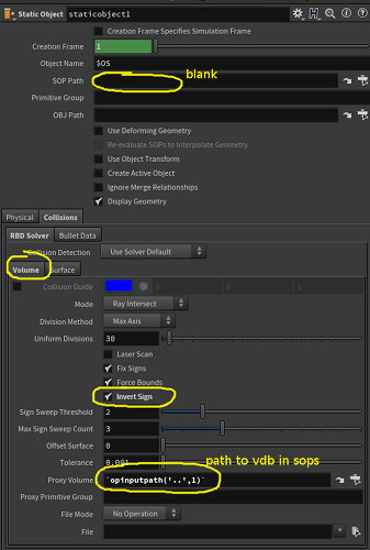
An easier solution is to make use of volume collisions. Easier still is to generate that volume in sops, and tell dops "don't make your own collision geo, just use this one I prepared earlier".

The trick is to use the 'proxy volume' parameter on the static object. You can turn on the collision guide to confirm its there, and in this case, use the 'invert sign' toggle to make sure dops knows to treat the inside of the sdf as empty space, not the outside:

Grains and hourglass ​

Download scene: hourglass.hipnc

Same as the above with animated sdf geometry.

Pyro ​

Pyro and collisions ​

Download scene: smoke_collide_pig_17_5.hip

Take that smoke pig! Now updated for 17.5, thanks to Charpentier Julien for asking me to do this.

The bottom pig is using the torus polygons as a (animated) static object collider. The top is using a sdf of the torus, and colliding using a volume source. You can see the results are pretty much identical.

When I first learned to do volume collisions I was told that using the regular static objects method to collide was a bad idea. A few months ago I watched a presentation by some sidefx folk, they're adamant that its fine, should work as expected without effort. You can see that's pretty much the case here.

That said, I've invested time and effort into learning the other way, I'll be damned if I'm giving up on it! I go into more detail below, but ultimately here the system looks for an sdf and a velocity field. When smoke is inside the sdf then smoke will be removed from the sim, and the velocity is used to update the sim to push smoke around.

Updating this setup to use the new volume sourcing workflow wasn't hard. Just create a volume source dop, use the preset combo box at the top to select collision, look for the volume names it expects (collision and v), make vdb volumes to match.

The advantage of using the volume method is more control; you can dial in how much velocity is transfered, by affecting the multipliers on the volume source dop, and often times production geo won't be well modelled, gaps and weird poly layouts can confuse the sim. If you can make an sdf and visually debug it so that it looks correct, you can be more certain that your end simulation will behave.

Whats needed for a pyro sim with collisions ​

These appear to be the basics required if you want to build a pyro smoke setup by hand.

• Sop level has...
  • a fluid source for the smoke shape
  • a fluid source for the collider (optional)
• Dopnet has...
  • a smoke object
  • a smoke/pyro solver
  • source volume for emission (optional)
  • a source volume for collision (optional)

Running through those in a little more detail...

• SOP, Fluid source smoke shape - where you convert a poly shape into a volume to either start the sim, or emit into the sim. Set 'division size' here to get the basic voxel resolution correct, and the density scale for the, well, density.
• SOP, Fluid source collider shape - same as above, but this creates an SDF for raw collision, and a velocity field (so make sure there's v feeding into this sop). To ensure its ready for collisions, on the container settings tab, set its initialise mode to 'collision'
• DOP, smoke object - the container for the fluid, home of the most interesting options, enough to break it into its own sub-list:
  • It has its own independent settings for the voxel res, so watch for that (often this is channel referenced to the sop fluid source or vice versa),
  • has its own size and center attributes. Annoyingly its hard to make it auto-resize on first frame without lots of hscript bbox commands, I tend to be lazy and set it by hand. This is easier to do visually; select the object, hit enter in the viewport, you get a standard box manipulator.
  • It also lets you set an initial value if you don't need an evolving or constant emitter (eg a static cloud). Properties tab -> initial data sub-tab -> density SOP path, point it to your fluid source.
  • Can set the boundary conditions, ie does the sim treat the container edges as solid walls, or does density just magically delete at the walls. Can set this for xyz, both positive and negative.
  • This is where you set what pyro attributes will be visualised, and in what format. Eg, you could turn on velocity, and make that display as streamer lines on a 2d slice.
  • To wire it into the system, connect it to the first input of the solver.
• DOP, smoke/pyro solver - where you set the time-step. The pyro solver is a beefed up version of the smoke solver, has extra handy tabs for shaping and adding turbulence and whatnot, I tend to use it by default.
• DOP, source volume for emission - point this to your fluid source sop, can set multiplier for density to be added per time step. It connects to the last input of the solver.
• DOP, source volume for velocity - point this to your fluid collision sop, it will inject velocity from that volume into your sim. It connects to the velocity update input of the solver (the middle one).

Scaling up a pyro sim ​

Download scene: pig_pyro_scale_v01.hipnc

After getting the previous test working, tried to make it completely from scratch without shelf tools, and make sure it worked at 10x scale, and 100x scale.

First, the fluid source sop for both the pig and torus use worldspace units to define voxel size. This means a size of 0.1 for a regular pig will make an unworkable number of voxels for a godzilla sized pig (easily into the 10s-of-millions). Adjust that first to make sure you don't bring houdini to its knees.

For the pig source, the resultant volume will turn spotty and horrible. You need to adjust the out feather length and density scale to compensate:

1. select the fluid source sop for the pig (NOT the one inside the dopnet!)
2. scalar volumes tab, SDF from geometry sub-tab
3. increase 'out feather length' until the volume looks natural again
4. the volume gets so dense that you can't see the form. use the scale slider next to density in the middle of the parameter window to reduce the density until it looks natural

Similar steps are required for the collider fluid source sop, but this time to make sure the velocity trail is accurately sampled. As the shape gets bigger, at some point the velocity isn't sampled at all, and you get odd collisions:

1. select the fluid source sop for the torus
2. get to a frame where the torus is in motion
3. velocity volumes tab, stamp points sub-tab, adjust the sample distance until you start seeing streamers again. They should broadly represent the collision geo.

Inside the dopnet, the smoke object won't resize itself, so do that first (a handy trick is to select it, and tap 'enter' while your mouse is in the viewport, you'll get a box manipulator).

Normally you'd also need to change the density slider here too, but in my example I've channel referenced it to get its value from the pig fluid source sop.

Pyro upres ​

Download hip: upres_v03.hipnc

5 years ago I wrote notes on uprezzing. I was so cocky that the workflow was so clear and obvious I didn't save a hip nor a gif. Every 6 months since then I've tried to recreate it, and failed.

I saw this demo and was determined to recreate it, couldn't. Finally today I asked some people, got an answer, saving a hip and gif here for posterity. Hooray, thanks Jeff!

The important bits:

• upres looks for a @timescale detail attribute, by default 1. If it doesn't exist, nothing works. A dopio node adds this, but you can do it yourself with a wrangle
• for smoke all you need is vel and density
• the upres solver dop requires a path to the input low-res sim, but it only uses @vel. You still have to add @density with a volume source (but you don't need anything else)
• that @density source can point to the output density of the low-res sim, but Jeff pointed out it works better with the density used as an input to the low-res sim. In the example you can use the dropdown menu on the source volume dop to swap between the first and second geometry, can see the difference in behavior.

In my case I tried to fake some extra vel detail with some volume wrangle tricks before feeding to the upres dopnet. Kinda works, kinda not. But hey, at least now this system actually does stuff.

Volumes, pyro, colour ​

Download scene: vol_col.hipnc

Update June 2017: There's useful info here, but be sure to check out the next example for a more up to date and cleaner method!

Strangely obtuse, but satisfying when it works. Like most of Dops. The high level summary is that you can make a volume primitive that contains colour easily enough, but nothing in houdini is setup to view it, or sim it, or view the sim. Setting it all up isn't hard, and its good I guess to learn how to wire in your own arbitrary volumes to pyro sims, but still, surprising that it doesn't 'just work'. So off we go; make a colour volume, visualise it, add it to pyro sim, make sure it gets simmed, visualise the sim.

Create a volume with colour ​

Getting colour into a volume is relatively easy. In this case I:

1. Made a grid
2. AttribFromMap to transfer colour into the grid
3. Extrude a bit to get depth
4. VdbFromPolygons to generate a volume, use the multilister to generate an extra 'Cd' volume, getting its values from Cd of the points.

Display volume colour in viewport ​

At this point came the first gotcha with volumes and colour; they don't display in the viewport by default. To do this requires a volume visualisation sop, with the diffuse slot set to load in colour (using the dropdown will set the correct attribute name as Cd.* )

So that's that. Getting it into a pyro sim is a little more work.

Import volume colour into a pyro sim ​

Starting from the basics of a pyro object and pyro solver, you'd expect to find a colour slot on the pyro object. Surprisingly, while it has slots to import density, vel, temperature etc, there's nothing for colour. As such, the Cd volume has to be manually inserted to the dopnet. This is done with a 'sop vector field':

1. Insert a sop vector field between the pyro object and the pyro solver
2. Set the sop path to the vdb (I like to use `opinputpath('..',0)` so I don't have to do explicit manual paths)
3. Set the data name to 'Cd'
4. Set the primitive number to '1 1 1'.

That last step was a little obtuse. A vector field in standard houdini volumes is stored as 3 scalar fields, so a Cd vector field is really 3 scalar fields named Cd.r, Cd.g, Cd.b. If you middle clicked on a volume, you'd see it listed as 3 primitive volumes.

The 'primitive number' field is where you'd enter the primitive id's of Cd.r, Cd.g, Cd.b. Assuming the colour volume was by itself, you'd enter '0 1 2'.

Because I'm using vdb's here, vdb treat vector fields as a self-contained primitive. Middle clicking on the vdbfrompolygons shows that the density volume primitive is 0, and the Cd vector field is 1. As such, we use '1 1 1' as the primitive id's. Clear eh? You should be able to middle click on the pyro solver and see that Cd is there.

There's a volume velocity sop to generate some swirly curl noise, which is pulled into the dopnet with a source volume dop (all modes on 'none' apart from velocity set to copy).

Affect volume colour with pyro sim ​

If the network was left in this state, you'd see the density get swirled around, but the colour would remain static, like an image projected into smoke.

To ensure the colour also gets swirled, a gas advect dop is used:

1. Create a 'gas advect field' dop
2. Connect it to the 'advect' slot of the pyro solver (it's the 4th input)
3. Set the field attribute to 'Cd', and leave the velocity attribute as 'vel'

Export colour from pyro sim, display ​

Now if you sim, the colour should swirl. Well it would if you could see it, but you can't. Again, there's no built-in support for colour within the dopnet, so you need to step back up to sops, import the Cd field from the pyro sim, and append another volume visualiser set to display Cd. Right then:

1. Get back up to sops
2. Create a 'dop import fields' node
3. Set the path to the dopnetwork
4. Set the dop node attribute to the pyro object, NOT the final output node. This really tripped me up for a while!
5. Add 2 fields to import, density and Cd. The mode doesn't matter, as we'll visualise it with the next sop.
6. Append a 'volume visualisation' sop, set the diffuse field attrib to 'Cd.*' as before, you should now see swirly coloured smoke.

Pyro and colour again ​

Download scene: pyro_cd_advect_v01.hipnc

While the previous example worked, it would behave strangely if I was emitting from a small source, or source via a source volume dop; the colour field would suddenly pop to white beyond a certain point, or refuse to be advected by velocity, or other strange behaviors.

Been toying this is for a while and pulled apart other peoples examples, I think I've nutted it. The most important and surprising lesson is this: don't use vdb vector fields for a coloured pyro sim. A lot of the weirdness I was getting (inverted colour channels, or only using a single channel, or clipping, or density being the opposite of the colour regions, or or or...) went away as soon as I put down a vdb convert sop before the sim.

The setup is largely the same as the previous example, with a few extra bits; a second volume source is used to bring in the colour info from sops (all I do is change the sop name fields so where it would normally bring in vel, I bring in Cd), the resize dop is told to also update the Cd field, and there's a gas diffuse dop to help blur the colour over time.

I also found an easier way to visualize colour within dops; on the smoke object set the display type to be only 'multifield', and you can set the displayed diffuse/vector field to be Cd just as you'd do in a volume visualise sop (the interface is nearly identical on that tab, I assume its the same under the hood).

Download scene: pyro_cd_advect_and_blur.hipnc

Another variation of the same thing, this time trying with much calmer forces and pulsed Cd emission to prove that it really was blurring the colours together. Found that a gas blur worked much better than a gas diffuse.

Pyro and colour yet again ​

Download scene: colour_pyro_more.hipnc

Every few months I revisit this, it gets clearer each time, the setup gets more streamlined.

This has a much cleaner sourcing setup courtesy the amazing Jacob Santamaria. This uses a gas wrangle, which to me feels much cleaner and easier to understand than the standard source volume dop.

The trick here is to mask the incoming Cd with a, well, mask, and lerp between the colour in the sim vs the colour in the source. No more fudging additive colour or struggling with how mixing in overlapping regions, just happy happy Cd.

The other trick cos I kept forgetting was the channel reference the dimensions and offset of the Cd field to match the smoke object. Several times I'd be shouting at colour going crazy, only to realise when checking the wireframe overlay that the Cd field was a 1x1x1 box at the center of the sim, and I never updated it. Dur.

Thinking about it some more, realized this is what a gas match field is for. Put that into the pre solve, tell it to make Cd match density, done. This means your Cd field is probably of much higher resolution than required, but my word it looks nice.

Add some disturbance, some tweaks to the sop sourcing, it gets very pretty:

Pyro and colour for the last time ​

Download hip: Pyro_colour_17_5.hipnc

Well, the last time before the next time. 17.5 updated pyro to have a more fully featured source volume dop, and the pyro solver and smoke object are now both aware of Cd by default, so way less manual wiring is needed.

As such, here's an updated setup. Note that I also finally worked out a neat trick from the Dop IO node that I didn't have before; vector fields usually look terrible in the viewport and obscure what you really want to see. Turns out you can change volume visualisation modes with a primitive sop, and set the visualization type to 'invisible'.

So, here's the summary:

• Sops pre sim
  • vdb from polygons, use it to get density and Cd
  • primitive sop to make the Cd field invisible
• Dops
  • In the sim, use a source volume, add an extra field to source for Cd, set its sop mask to 'density' so that it doesn't flood the rest of the sim where it's not required
  • An advect field dop is used to push Cd from vel
  • The smoke object display mode is set to multifield with density and Cd
  • Density and Cd are exported from dops back to sops
• Sops post sim
  • Cd made invisible again with primitive sop
  • Converted houdini volumes to vdb, vector merge Cd
  • Primitive sop used to compress to 16 bit vdbs to save space
  • Exported with a filecache to a vdb sequence

Pyro and colour in H18 ​

Download hip: pyro_sops_with_cd.hip

Of course the last time wasn't the last time. This is the last time. Until the next time.

The setup is actually mostly the same as the previous attempt, but the biiiig difference is this is using the new pyro-in-sops workflow. No FX license needed! No playing around in icky dops!

The main thing you need to do here is make sure Cd is being advected. On the pyro solver sop, solving tab, advanced sub-tab, advection sub-sub-tab, add 'Cd' into the 'extra fields' section.

Advect smoke with particles ​

Download scene: advect_smoke_with_pops.hip

First part is simple enough, a small pop setup that fires a handful of particles every 2 seconds. The location pop is good for simple things like this that don't require any source geo; just give it a position in space and it'll birth particles for you. There's an hscript expression on the const. activation parm:

if($T%2<0.5,1,0)

Ie, loop time ($T) every 2 seconds, if its under 0.5, fire particles, otherwise don't. The attributes tab sets the initial velocity, which is +Y, plus a lot of variance (randomness) in all directions to get a burst in all directons. It then uses a replicate pop to emit a short trail of extra particles behind the primary particles.

Next is the smokey part.

This base sim is even more basic than the previous examples; a smoke object and smoke solver. The two interesting extra nodes are the gas 'particle to field' dop and the 'fetch data' dop.

Particle to field does as it says, reads particles and converts it into a volume field. Here, we read 'v' from the particles, and convert it into 'vel'. It's set to add to the existing vel, so it can accumulate.

I thought this would work as-is, but the particles refused to affect the smoke at all. First I tried changing the geometry name it was looking for, then gave it a full path the particle object, still nothing. Gave up and asked our dops wizard, who pointed me at the fetch data dop.

Even though I had the particle sim and smoke sim merged together, the smoke sim had no idea that the particle sim was there. It has to be explicitly brought into the smoke solver, hence fetch data. The geometry spreadsheet confirms this (once you know where to look), if you expand the smoke section, there's no 'Geometry' entry until you use the fetch data dop.

The nodes after the dopnet are to process the raw smoke data into something interesting. The raw sim looks like a steamy room, with people throwing basketballs around inside to move the steam. Instead, I convert the houdini fields to vdb fields (easier to manipulate that way), and set density based on vel. Low vel = no density, high vel = lots of density. This changes the look from steamy room to missile trails.

I have a better version of this in the longform tutorial SmokeDetailed.

Advect smoke with particles via vdb ​

Download scene: pyro_vortex_from_pops.hip

Download scene for H17.5: pyro_vortex_from_pops_17_5.hipnc

Same idea as before, but this time using a more traditional 2 part approach:

1. do the particle sim first, convert to vdb
2. use that vdb as a source volume for a pyro/smoke sim.

This tends to give smoother results, and be a little more controllable, which may/may not be what you want. I found applying this technique to the missile trails looked too smooth. I found inserting a volume vop between the vdb's particles and before the pyro dopnet, and adding curl noise to vel, helped take away the smoothness, but at least now I know two ways to skin this cat.

Dylan Smith emailed me to point out a gotcha with this setup. Similar to how a 'vdb from polygons' sop will make a density field that is dense near the polys, and fade towards the center of the shape, a 'vdb from particles' will essentially treat each particle as a sphere, and transfer velocity/density/whatever at the edges of those spheres.

This means if you're trying to be efficient and use a large particle size, in this example you'll get an inner and outer 'wall' of velocity where the particles are all conforming to the tornado shape, with an empty groove in the middle. You can compensate for this by using a smaller particle radius, or making sure your particles are chaotic enough that the don't align enough to form channels, but something to watch for. Thanks for the tip Dylan!

More advecting smoke with particles (aka pyro blendshapes) ​

Download scene: pyro_blendshapes.hipnc

The result of seeing a nice video of particles that blendshape into various states, and then seeing another video of a pyro/particle wisp thing, this is a blend of the two.

1. Multiple shapes are fed to a keyframed switch sop, followed by a scatter that generates 2000 points.
2. A point generate is set to make 2000 points, and is fed as the source to a pop sim.
3. Pop sim is in 'all points' mode, and only generates particles on the first frame
4. A pop attract is used to goal the particles to the scattered points, drag is used to keep it from going crazy (feels like there should be a cleaner way to do this...)
5. Outside the popnet, particles are fed to vdbfromparticles to generate a volume source for the next section
6. A second dopnet is used for a pyro sim. The particles are brought in with a 'sop geometry' dop, and their @v converted to @vel with a 'gas particle to field' dop. Messed around with this to determine the right mode for the vel transfer, in the end just an 'add' mode looked pretty cool.
7. All rendered via the opengl rop, which I'm pleased to say worked quite well and is quite fast.

Pyro stick to surface with project non divergent sop ​

Download scene: pyro_stick_to_surface.hip

A work in progress, but liking where this is headed.

Someone on discord asked how to swirl pyro around a shape. In my head this seemed simple enough; do one of the cross tricks to take the object normal, cross it with another vector (noise or a world axis), which gives you a vector along the surface of the shape, feed it to a pyro sim.

In practice, pyro would quickly drift away from the surface. My next intuition was that you'd need a multiplier that would increase with distance from the surface, forcing vel back towards the surface. Using an sdf of the surface seemed a good way to do this:

// vdb prim 0 is the sdf of the surface
float sdf = volumesample(0,0,@P);
vector grad = volumegradient(0,0,@P);

// vector towards the surface, that reduces close to the surface
vector inforce = -sdf*grad;

// blend the original vel to this inforce, based on distance to surface
@vel = lerp(@vel, inforce, abs(sdf));

// vdb prim 0 is the sdf of the surface
float sdf = volumesample(0,0,@P);
vector grad = volumegradient(0,0,@P);

// vector towards the surface, that reduces close to the surface
vector inforce = -sdf*grad;

// blend the original vel to this inforce, based on distance to surface
@vel = lerp(@vel, inforce, abs(sdf));

Applied it and... not bad, but not great. Occasionally the smoke would form tendrils that would shoot off from the surface, ruining the read of the shape.

In hindsight, this is probably the pyro solver project non divergence doing its thing. The velocity from the wrangle inherently had some areas where pressure build up was too great, other areas becoming a vacuum, so pyro naturally tries to balance those, which would create local high pressure channels of velocity for the smoke to escape from.

At this point I remembered a recent addition to the vdb toolkit; vdb project non divergent. This does as the name implies, it iteratively tries to solve divergence in a velocity volume. Applying it to my volume, it warns that it couldn't solve all the divergence but that's ok, it solved most of it. Feeding that to the pyro solver behaves a lot better, as the forces are now much more stable. Occasionally there'll be little escape wisps, but that's fine, it keeps the smoke overall looking natural and interesting.

The pig head is a worst case example, the sharp kinks in the surface mean the smoke won't have much of a chance to follow the shape. A sphere works rather well, and doesn't require any of the more common cheats like multiplying density down based on distance to the surface, or high dissipation, or other stuff.

Pyro detailed smoke ​

I broke this out into its own page as it got a little long, you'll find it on SmokeDetailed.

Pyro 2d solver ​

Download scene: 2d_fluid_soap_bubble.hip

Super fun, super fast, this solves at around 18fps on my workstation. It's mentioned elsewhere, but all you need to do is enable the first checkbox on the smoke object for 'two dimensional'. I've also deleted the output node so its not trying to cache to disk, and enabled openCL on the solver to get it nice and fast.

A happy byproduct of this is that its very easy to play with the shaping controls on the pyro solver, and see what they do in nearly realtime. Turn off everything but confinement, set it to 1, sim, 10, sim, 100, sim. Turn that off, turn on disturbance play with the scales and thresholds, turn on sharpening, overdrive it, etc... I learned more in 10 mins this way about what the various controls do than in the last year of using the pyro solver!

Pyro divergence and sinks ​

Download scene: pyro_divergence_sink.hipnc

Lovely example from Henry 'Toadstorm' Foster. A key reason pyro sims move as they do is that pressure and volume is maintained, causing all the fun swirly smoky goodness. If you throw a few more fields in mix, you can get some very interesting effects.

A sink field removes density, in this setup the sink source volume is set to 'clamp sub', so that it subtracts density towards the center of the sim.

Divergence is used internally to calculate where there's positive or negative pressure building up. Pyro will try and balance divergence (the step goes by the easily remembered name 'gas project non-divergence'), so that focal points of add/suck become swirly centers instead. You can override this by adding your own divergence, here again its set to have negative divergence, drawing the volume motion towards the center of the sim.

I felt compelled to do some value add, and showed how you can use a volume vis node to remap the density into a eye-of-Sauron look. Thanks for sharing Henry!

Tornado ​

Download hip: tornado_from_curves_v04.hipnc

Yet another thing I try every few months, but the first time I've been pleased with the end result. Had a look at Ben's great tutorial from a few years back, but was curious if I could avoid vex and vops here, and just construct it out of vanilla H18 nodes, and the sop pyro solver.

I make a spiral of tubes, add some animated noise, and use it to create a density field and a vel field. The vel field uses the handy volumevelocityfromcurves sop, with a bit of help from a polywire+sdf+convert to polys to give a rough surface skin to the tornado shape, which helps the volumevelocityfromcurves do its thing. A volumevelocity sop adds some extra noise. Meanwhile to make the density I do some bound and tube tricks to make a little disk that tracks to the bottom of the curves, and add some cloud noise to create some interesting shapes. I caved and made a little vex wrangle to convert this disk of density into a ring of density.

These are merged and fed into the pyro sop, where there's not much extra happening. Vel is boosted substantially, as is density, disspiation is tweaked to make sure the shape stays readable. Inside the solver I added a disturbance node to rough it up a little, but that's it.

What surprised me is how fast and violent this looks; normally when I've tried pushing vel really hard the sim starts to get dotty, stepping becomes visible, it all looks ugly. Similarly I've never had much luck with sourcing vel in 'copy' mode, I've always used 'add' or been careful with masking. Here it's just the default 'copy'. looks pretty good.

2d wind tunnel ​

Download scene: pyro_wind_tunnel.hip

Paul Esteves asked about a setup like this, I had a go, Lewis Taylor suggested I upload it.

The setup is pretty simple by design; generaly I find the more I can get away with static inputs to the pyro sop solver, as few fields as possible, and turn off all the internals, it runs much faster.

The right-to-left motion comes from shapes -> wind, expanding that section and set the direction to -1 on X.

The nice eddies and disturbance come from using a collision and collisionvel sdf. The vel is set from normals of the collider sphere, but in sourcing I've multiplied it down by 0.3, otherwise the wake is too wide.

Extra eddies are setup by enabling advection-reflection on the setup tab. Try disabling it; the sim runs a little faster, but the wake isn't as interesting.

Rigid Body Dynamics ​

RBD and packed prims ​

Download scene: rbd_pig.hip

To set this up by hand to get a Deep Understanding, there's 4 main things:

1. scatter points within the shape to drive the voronoi fracture
2. voronoi fracture, convert the fracture to packed prims with an assemble sop
3. setup forces if required
4. create dopnet with rbd packed object and rigid body solver

This uses a trick I don't think is written down on the wiki yet, but is used a lot; feed scatter a shape, it generates points on the surface. Feed it a volume, it scatters points throughout the volume. Thus, if you need to scatter points inside a shape, convert it to a volume, then scatter. A shape can be converted to a volume in several ways, the usual 2 options are the IsoOffset sop, or the VDB from polygons sop in fog mode.

I made a silly mistake when setting up this example, I used the tab menu to look for 'rbd solver', took me a while to work out that's the wrong one. You actually need a 'rigid body solver'. The sheer amount of nodes available in Houdini is both a blessing and a curse. 😃

RBD lo-res packed geo, apply sim to hi-res packed geo ​

Download scene: rbd_pig_v02.hip

Same explodey pig as the previous example, but with a shape replacement workflow (with caveats, read the next section...)

1. Unpack the geo in a separate branch
2. Add detail in whatever way you want (I used a subdivide and mountain)
3. Pack again (optional, the information needed in the next step is still there in the @name attribute, but packing is neater)
4. Use a transformpieces sop, high res geo on the left, lo-res sim in the middle, it will transfer the animation from the lo-res to the hi-res.

RBD extract correct transform attributes ​

I had to use a variation of the above trick in production; I had very high res packed geo, so I generated my own low res packed proxies, ran a rbd sim, and used transform pieces to copy the animation back to the high res geo. At a glance it was fine, but in dailies on a big screen something was off; objects were slightly misaligned, pivots incorrect, strangeness.

Rubens Fredrick pointed out the problem; the orient/scale/pivot point attributes that come out of a packed rbd sim are often incorrect, and can't be trusted. Instead, you have to go directly to the intrinsic attributes of the primitive itself, and rebuild the correct point transform attributes:

matrix m4 = primintrinsic(0,'packedfulltransform',@ptnum);
matrix3 m3 = matrix3(m4);
@orient = quaternion(m3);
@scale = cracktransform(0,0,2,0,m4);
v@pivot = primintrinsic(0,'pivot',@ptnum);

matrix m4 = primintrinsic(0,'packedfulltransform',@ptnum);
matrix3 m3 = matrix3(m4);
@orient = quaternion(m3);
@scale = cracktransform(0,0,2,0,m4);
v@pivot = primintrinsic(0,'pivot',@ptnum);

I've since had other co-workers say that even this can't be trusted, and sometimes you need to refer to other intrinsics. If anyone has a definitive answer I'd love to hear it!

Emit packed prims into RBD sim ​

Download scene: emit_packed_rbd.hip

Super clever setup courtesy Tomas Slancik. As outlined in this odforce post, I'd worked out how to emit packed objects in a naive way, but it got very slow very quickly. A tip on the forum revealed another method, but I had a hunch that while performance was much improved, the setup was a bit clunky.

Tomas to the rescue! The trick here is that a packed shape is basically a point. A pop source emits points, so we can use it to emit shapes into an rbd sim. The main thing to watch for is that its emission type is set to 'all geometry'. This, like the differential growth example, does what its told, and just feeds whatever you tell it into the sim.

The other trick is to that the 'rigid body solver' already has a multisolver built in, so all the extra work I was doing in the forum post examples isn't needed here.

Because I felt the need to value-add, I tweaked Tomas's setup a bit to show how it can emit multiple packed shapes.

Emit packed prims and randomly activate ​

Download scene: rbd_random_drop.hip

Moving up the scale of contrived demos, inspired by a question Beck asked, cheers Beck!

Pops give you a nice lazy way to scatter emission over a shape. Making a similar thing with packed rbd is a little tricky. To make things harder still, I wanted this to emit random rbd objects, and to randomly activate after a short delay.

Packing the shapes is easy and is basically the same as the previous setup, with the added bonus of fixing the @name attribute. For the simple emit example earlier it doesn't matter, but when you start working with constraint networks (covered shortly), or do fancier things to the packed geo in dops, duplicate names can break things.

Here I'm copying shapes to the results of a scatter sop, so I setup all my attributes in a wrangle immediately after the scatter. To set the name I construct a string from the ptnum and the current frame, using the sprintf function to do some C-style formatting. I can write 'my_cool_%g_name_with_%g_numbers', @ptnum, @Frame, and the %g will be replaced with the variables I specify, in the order I specify. So with the following vex code...

@name = sprintf('piece_%g_%g',@ptnum,@Frame);

@name = sprintf('piece_%g_%g',@ptnum,@Frame);

...point 12 at frame 5 will get the name 'piece_12_5'.

This will copy all the packed shapes to each point, obviously we want a single random packed shape per point. This is yet another attempt to do this cleanly, not sure how well I've done. Because each cluster share the same name, I can run a foreach loop on name, randomly sort, then keep the first one I find.

Devil is in the details of course. Initially I set the loop to run on points, using the name attribute. It works, but it also deletes the packed prim info, which is no good to us. To get around this I promote the @name attribute from point to prim, then set the loop to run in prim mode.

The randomizing is done with a sort sop, to my surprise it sorted every prim cluster identically, which if you think about it, makes sense. It has to be repeatable randomness, otherwise we couldn't get anything done. As such, the seed for the random sort has to be driven from the loop, so I use a metadata node to get the iteration, and use a spare input to pull that into the sort seed.

Finally inside the dopnet I do the random activation. This is a geo wrangle, where I increment an @age attrib per frame, and test it. The scattered points have @active set to 0, this code will randomly turn active to 1 after the points are older than 10 frames:

@age++;
if (@age>10 && rand(@ptnum)>0.5) {
  i@active=1;
}

@age++;
if (@age>10 && rand(@ptnum)>0.5) {
  i@active=1;
}

RBD packed prims and deforming geo ​

Download scene: pig_deform_to_timed_rbd.hipnc

Full credit goes to wateryfield on the odforce forums: http://forums.odforce.net/topic/24604-deform-rbd-sim/?p=143902
Bonus credit to Vladimir Lopatin for the tetris brick voronoi fracture trick: http://forums.odforce.net/topic/22175-brickstone-wall-broken-horizontals/?p=143621

A few subtle differences in this setup compared to the previous one that creates a fun end result:

• Voronoi fracture as before, but using a grid of points that have been clustered rather than a scatter. This creates the tetris style pieces.
• Twist deformer to do the head shake
• Wrangle that sets @active to 1 in a timed way from top to bottom, and @deforming to always be the opposite of @active.
• In the dopnet, rbdpackedobject has just 2 things modified:
  • The initial object type is set to 'create deforming static objects'. Ie, bring in the deforming mesh, don't do any simulation on it.
  • The overwrite attributes toggle is enabled, meaning it will read in @active and @deforming from the incoming geo.

As you'd expect, if the packed chunks have @active=0, the rbd sim doesn't touch them. Also as you'd expect, if @deforming=1, the sim will also load the deformed chunk. When those states are swapped, the piece will stop deforming (it will be in whatever the last deformed shape was), and will start to fall and collide driven by RBD.

We can all look forward to being hired for a Buffy/Blade sequel now (assuming all vampires are pigs).

RBD inherit @v and @w after initial frame ​

Download scene: rbd_inherit_v_after_initial_frame.hipnc

September 2017: Someone pointed out that Houdini now behaves as expected, and no longer requires the solver+wrangle workaround outlined below. Skip to the next chapter to see a setup that incorporates this.

Had posted this on odforce a while back, forgot I never put it here...

Using packed RBD makes sims easier; set their @v (for initial velocity) and @w (for initial rotation) like in the earlier examples, run the sim, awesome. But what if you want to stagger the timing of their @active state, like in the gif above? Well, that gets slightly complicated. The packed rbd object has an option to inherit point attribs, but if you try and use @v and @w after the first frame of the sim, it gets ignored.

The reason is that the packed RBD solver itself uses @v and @w, so it'll just ignore your point values. My initial reaction to this was 'fine, I'll add a wrangle in a solver, and force the sim to read @v and @w'. The result was pieces flying away to the edge of the universe, which is no good. Turns out that setting @v and @w from the initial geo, on every frame, makes the RBD solver go crazy.

The attached scene provides a solution. Rather than just blindly set @v and @w every frame, it checks the @active state compared to the previous frame. If a piece has just been made active, it reads @v from the incoming geo. Otherwise, it does nothing, and lets the RBD solver do its thing.

Oh look, a slightly better version of the same thing! Done in H16 just to check I could remember how to do it (I could), and to come up with a more interesting pattern (a curve to drive the voronoi fracture, and a point travelling down the curve to trigger the chunks):

Download scene: staggered_fracture.hipnc

RBD inherit v revised, plus orbit ​

Download scene: rbd_orbit_staggered_emit.hip

So as of mid 2017, H16 packed RBD now behaves as expected, and will inherit v from the source geo for the first frame it's active, which is much nicer. To make this example a little more interesting, this setup uses a pop axis force to swirl the pieces into an orbit. If used by itself the pieces will fling away too quickly, so a pop speed limit is used to clamp their speed, locking them in orbit.

RBD follow targets ​

Download scene: rbd_targetp.hip

I got goaded into trying this, damn you twitter.

I assumed packed RBD would support targetP, it doesn't. Looked at the docs, there's targetv, tried that, didn't really do what I wanted. Caved and looked at odforce, was surprised to see that just setting @P from an external reference works. However if you look closer, you can see that while the pieces still rotate from the sim, the position is totally driven by the input, which wasn't quite right. Instead I tried the other technique of calculating @v by subtracting the current rbd position from the input target in a geo wrangle. By default it completely softens the motion into a bland mess.

The lazy answer is to just multiply @v until it starts to look peppy again. Have to dial this in though; too much and it overshoots, too little and its bland, and then you have to mix and balance again if you add extra forces and collision geo like I've done here.

The right answer of course is to use constraints and springs and stuff. I have a longer tutorial for that here: ConstraintNetworks2, but this cheap and cheerful setup works pretty well.

RBD follow targets v2 ​

Download scene: cube_walk_rbd_targets.hipnc

Here's another take on the same thing, with bonus tricks to try and find the closest point on the surface first, then when within a threshold try and seek the proper target position.

RBD deintersect via scaling up geo ​

Download scene: rbd_deintersect_via_scaleup.hip

Make sure to read the next entry, 'RBD deintersect the easy way', leaving this here cos it seemed clever at the time...

Thanks to Jake Rice for the idea! By scaling rbd objects from 0.1 to their final size, but keep them constrained where they're meant to be, they'll naturally collide and de-intersect themselves. The trick is to make sure the object scale can be cleanly controlled, while letting position and rotation be driven by dops, and the collision shape be correctly updated while growing. In this case the positions are locked, so I'm only dealing with the scale and rotation.

I have an attribute @s, that I've keyframed from 0.1 to 1 quickly at the start of the sim.

A geo wrangle in the dopnet composes a new transform on each frame using the rotation from dops, scale from sops, with scale multiplied by the @s attrib, then that transform is pushed back onto the shape. The wrangle looks like this (the first context geo on the wrangle is 'myself', ie dops, the second context geo is the first input to the dopnet).

if (@Frame<20) {
    matrix3 dt = primintrinsic(0,'transform',@ptnum);
    matrix3 st = primintrinsic(1,'transform',@ptnum);
    vector r = cracktransform(0,0,1,0,dt);
    vector s = cracktransform(0,0,2,0,st);
    s*=@s;
    matrix3 m = matrix3(maketransform(0,0,0,r,s));

    setprimintrinsic(0,'transform',@ptnum,m);

    @id=-1;
}

if (@Frame<20) {
    matrix3 dt = primintrinsic(0,'transform',@ptnum);
    matrix3 st = primintrinsic(1,'transform',@ptnum);
    vector r = cracktransform(0,0,1,0,dt);
    vector s = cracktransform(0,0,2,0,st);
    s*=@s;
    matrix3 m = matrix3(maketransform(0,0,0,r,s));

    setprimintrinsic(0,'transform',@ptnum,m);

    @id=-1;
}

Setting @id to -1 forces bullet to recalculate the collision geo per frame, note that I'm only running this for the first 20 frames, ideally this would be done in pre--roll before the shot.

In hindsight I probably don't need it to be this fiddly, as all my shapes were of scale 1 anyway to start with, so just taking an identity matrix for scale, then multiplying by @s would have been fine. Still, if I had incoming packed geo with pre-existing random scales, I'd be ready. 😃

While this works pretty well, it feels like there must be a better way to untangle rbd objects. If you know a method, please get in touch!

RBD deintersect the easy way ​

Download scene: rbd_deintersect_simple.hiplc

Well someone did get in touch, Paul Ambrosiussen. He pointed out a much easier way; just set

 i@found_overlap=1;

 i@found_overlap=1;

On your packed shapes. You can even try turning on 'solve on creation frame', and if there's enough space then your shapes will deintersect immediately. In my leaf example it still needs a few frames, but still, much easier than my matrix work from earlier. Thanks Paul!

Update v18.5!

There's been a collection of sops to help make constraint systems since around v17, I've only gotten around to playing with them properly since v18.5. They're on their own page, I've added an improvement to this deintersect system over there: https://www.tokeru.com/cgwiki/index.php?title=ConstraintNetworks3#Constrained_deintersect

Update v19.5!

The bullet/packed rbd solver in 19.5 has had many quality-of-life improvements, a key one being it now properly reads animated instance attributes on input geometry. This means you can just animate @pscale or @scale, the rbd shapes will update, no need to use the @found_overlap trick which can be very expensive on big sims.

RBD reapply packed anim to RBD packed shapes ​

This section is mostly superseded by the new 'transform by attribute' sop in H17.5. Oh well.

I have some animated packed geo. I want to export it via the 'rbd to joints fbx' tool from the gamedev shelf. If I try, it complains about something, apparently my packed geo doesn't have the same attribs that a rbd packed sim, something under the hood is breaking.

To be cheaty, I just run my anim to a packed rbd sim so it creates the right attributes, and timeshift it to lock the first frame. Now it has the right attributes, but I need to copy the original animation back onto these pieces. Make a point wrangle, frozen rbd sim to input0, packed anim to input1:

matrix pft = primintrinsic(1,'packedfulltransform',@ptnum);
setprimintrinsic(0,'transform',@ptnum,matrix3(pft));
@P = cracktransform(0,0,0,0,0,pft);

matrix pft = primintrinsic(1,'packedfulltransform',@ptnum);
setprimintrinsic(0,'transform',@ptnum,matrix3(pft));
@P = cracktransform(0,0,0,0,0,pft);

This is a variation on the previous example, but this time completely dispensing with the orient and scale stuff. If you have animated packed prims (either from rbd or hand keyed), all the animation is maintained on the 'packedfulltransform' intrinsic. If you have point @orient and @scale, they might be updated, but thats a convenience, and not guaranteed. You can prove this by putting an attrib delete down and blasting all the point attributes; you might have to click somewhere else and click back, but now you'll only have @P, yet the packed geo will still be rotating and scaling away.

So really, what we need to do is copy what packedfulltransform is doing onto our frozen rbd geo. But remember that packedfulltransform is a read only intrinsic. Ugh.

As such, you need to break it out to a matrix3 and apply that the the 'transform' intrinsic we can write to, and extract the translate component of that and apply it to @P.

After writing most of the above, I thought 'hang on... isn't transform and @P from the original geo also kept up to date with packedfulltransform?' And yes it is, so you can rewrite it in this slightly simpler way:

matrix3 t = primintrinsic(1,'transform',@ptnum);
setprimintrinsic(0,'transform',@ptnum,t);
@P = point(1,'P',@ptnum);

matrix3 t = primintrinsic(1,'transform',@ptnum);
setprimintrinsic(0,'transform',@ptnum,t);
@P = point(1,'P',@ptnum);

Same thing, but again I recall some people pointing out that in some cases they won't match (packed alembics I think), so good to know both forms in case one breaks.

RBD in 17.5 ​

Download hip: rbd_17_5_simple.hip

17.5 introduced a new RBD workflow, influenced by the way vellum combines geo and constraints. There's a fantastic in depth 2 hour masterclass by Cameron White, this is a summary of the raw basics. More to come as I need it. 😃 So then, if you're used to the previous workflow, here's the crib notes:

• material fracture is an fancy HDA that'll scatter points, fracture, add edge detail, give a choice of concrete/wood/glass fracture patterns, and make a constraint network, all in the one node.
• material fracture can feel a little slow compared to voronoi fracture, but its doing a lot under the hood (take a peek)
• like vellum, the idea is for geo and constraints to flow together with the new multi-in-multi-out sop nodes
• rbd_constraint_thing nodes are like vellum constraint nodes, they can modify existing constraints or create new ones
• surprisingly it doesn't pack the geo for you, you need an assemble sop on the geo stream just before feeding to the dopnet (with 'create name attribute' disabled)

There's loads more, again watch the masterclass, but this is enough for a quick intro. Note that previous workflows for RBD are still valid, so don't panic and change over all your setups if you're in the middle of a project!

RBD sphere collisions from vdb ​

Download hip: rbd_spheres_v05.hipnc

A trick a few folk use to get fast lazy collision is to convert shapes to a vdb sdf, then use the vdb to spheres sop. Bullet can use sphere primitives directly for collision. If all the spheres that belong in a single object share the same name, then bullet will treat the spheres as a single object.

Here's a little setup to do all that as automatically as possible. A bunch of shapes are thrown together, and a for loop is run per connected piece. Each piece is converted via the vdb to spheres sop, and the connectivity @class attrib is used to construct a @name. This is fed to the rbd sop solver, and by using the handy hero geo inputs and the proxy geo inputs, the rbd motion can be directly applied to the original geo.

RBD coin follow path ​

Download hip: rbd_roll_along_path_v04.hip

Challenge from a friend, with some tips from Nick Taylor and a few folk in discord.

This is basically the same constraint network setup used in ConstraintNetworks2, with Nick's trick of using a pop lookat to steer the coin along its velocity.

There's a few more things in there (a wrangle to stop the coin vibrating at the end, a drag spin to help calm the motion a little), while it works it all feels a little over complicated. Anyone know of a cleaner way of doing this?

RBD replicate ​

Download hip: rbd_replicate.hip

Pingo van der Brinkloev got in touch and asked how you'd do a Harry Potter style RBD replication thing. Here's a quick setup I came up with, which he turned into three nice ads about recycling.

Bullet RBD lets you add objects whenever, the trick here was to control where it happened, and make sure no name collisions occured. I use a sop solver in dops to drive this, a metaball intersects with the rbd shapes and transfers a replicate attribute. When this happens, the tagged shapes get their name modified to include a new random number, and are merged with the original rbd shapes.

Some stuff added to control the randomness of replication, and added forces, its fast to sim, easy to control.

RBD panchinko ​

Download hip: rbd_glow_pachinko.hip

Question on reddit that I thought I'd have a go at.

The blockers are created using scatter and align, fast way to setup the random rotations of the platforms.

The emission driven by a plane and a scatter that has its seed randomised every frame. A sphere is copied to the scatter points, and that's used as a source to an rbd solver. The blockers are fed in as collision geo, with extra planes on the front and back to keep the spheres from bouncing too far away.

Within the rbd solver I have a geometry wrangle that removes objects if they go below P.y = -1.

The fun stuff was making the blockers light up when they get hit. I knew from earlier attempts that bullet allows you to access impact data, but vaguely recalled it was tricky. Hoped that the rbd solver sop had made this a little easier.

It does! There's an 'impacts' tab, with a 'fetch impacts' button. Click it, it makes an object merge that extracts the impact data from deep in the dop network, and pulls it up to sops. Nice.

Except... it didn't seem to do anything. After playing with it a bit, I realised the impact threshold parameter need adjusting. The tooltip implies its a threshold for breaking constraints, but lowering it from 100 to 10, and making sure 'show impacts' was enabled on the visualise tab, I could see the hardest hits would generate a point. Lower it to 5, and I got more hits. 2 seemed to be a good number.

These generated points hang around forever though! I needed the impact just for a frame or two when they first hit, then needed them to go away. The impact points record their time of impact, so I just compared that against the global time, and if the difference was too great, delete them:

@a = abs(@impacttime-@Time);
if (@a > 0.2) removepoint(0,@ptnum);

@a = abs(@impacttime-@Time);
if (@a > 0.2) removepoint(0,@ptnum);

I could then have the blockers test if a impact point occured near them, and if so boost their colour:

i@a = nearpoint(1,@P);
vector pos = point(1,'P',@a);
@d = distance(@P, pos);
if (@d < ch('cutoff') ) {
  @Cd *= 50;
}

i@a = nearpoint(1,@P);
vector pos = point(1,'P',@a);
@d = distance(@P, pos);
if (@d < ch('cutoff') ) {
  @Cd *= 50;
}

Worth noting this was the second method I tried. The impactpoints have an @impactprimnum attribute, that seemed the most obvious way to directly link impacts to the blocker shapes, but when I did that the prim numbers didn't match up. Using nearpoint is hacky, but works well enough here.

I also wanted the colours to fade rather than just blink on and off. I did this using a solver sop, using one of the standard techniques for transferring colours from the previous frame, then multiplying down by an amount on each frame.

Finally added some viewport glow for extra pizazz, display options, fog tab.

Another curious thing to be aware of; if I just displayed the object merged impact points, I'd get nothing at all. If I visualised the impacts on the rbd solver, they'd be there. If I swapped from viewing on the rbd sovler to the object merge, the points would stop being generated at the time I swapped! Feels like a bug to me, kind of like being inside a solver sop while displaying it. I learned to to turn on viewing the impact points on the rbd solver first, let it run the entire frame range, then I could swap to the object merge, OR make sure to view the final merge of the rbd spheres AND the glowing blockers. I suspect having the spheres displayed at the same time triggers the correct chain of dependencies, and stuff works again. Silly RBD.

Constraint networks ​

Here's some quick examples, I go into more detail in the longform tutorial ConstraintNetworks, and then more into animated constraint networks in ConstraintNetworks2 and ConstraintNetworks3.

RBD packed prims and constraint networks ​

Download scene: dop_glue_v01.hipnc

You can create edges between packed prims, and tell houdini to treat those edges as constraints for RBD. Further, you can manipulate those edges and their attributes in sops, and dops will do its best to follow along. The example scene is well annotated, but here's the workflow anyway:

1. Create packed-rbd setup as per previous examples (fuse sop in unique mode, assemble sop with pack enabled, dopnet, rbd packed object, rigid body solver)
2. Connect adjacent pieces sop, for the first time in these wiki/houdini experiments using it for its original purpose. It looks at the packed geo, and creates edges between them (it removes the original packed geo too)
3. Set attributes on these connection edges to set @constraint_name as 'glue' and optionally @constraint_type and @strength.
4. In the dopnet, append a constraint network dop, point it at your connection edges
5. Create a glue constraint relationship dop, it connects to the green input of the constraint network
6. Set properties here, and make sure its data name is also 'glue'. This is how houdini matches the incoming connection edges to this particular constraint, and builds the network.

In this example I randomly set the @strength attribute of the edges from 80 to 0.1, which breaks the glue connection and collapses the shape. Talking to colleagues and even the official help pages confirmed what I suspected; if folk can do the setup and interesting animation effects in sops, they'd rather do that, and leave dops only for the actual simulation work. It'd be possible to do this stuff using extra solver sops within dops, but its just easier to keep as much stuff as possible higher up in the sop context.

Constraint network rolodex ​

Download scene: rolodex.hipnc

Interesting question from the sidefx forum, thought I'd post my answer here with a mild tidy up. I explain more in ConstraintNetworks2, but the idea here is that you can setup constraints by making your own polylines. If points on the polyline have a @name that matches the @name of your packed shapes, they'll be constrained together. If the other point on the polyline has a @name with an empty string, you can animate those points, and it will drag the packed shapes with it. The details are subtle and tricky at first, this is a good clean example to work from.

Constraint networks, quick visual reminder ​

First time I dove into these they seemed a little complex and arcane, but once you understand the idea behind it, its not too bad. Here's a simple, uninteresting dop network; packed rbd, going to a solver, gravity, output:

Here I add a collision setup, which you could think of as its own little network. Just a ground plane, static object, and linked to the sim with a merge.

I've used colour to group the related nodes; the rbd nodes are one thing, the collision stuff is another, gravity is its own thing. Constraint networks are also their own form of network, that get wired into the overall chain. First, the constraint network relationship node:

This node needs a sop path to the constraint edges you'll make (most likely with a 'connect adjacent pieces' sop). But here, even with that path filled out correctly, it errors, which confused me. The reason is that it must have another input to it, in this case, a glue constraint relationship node:

Aha! No more errors, network is happy. The reason is that while the constraint network relationship node pulls in the constraint edges, it doesn't know what those edges represent. Thats the job of the 'glue constraint relationship' node, to create the type of constraint you want, and the strength and properties of those constraints.

To make it clear that these are separate kinds of networks (ie, rbd network vs collision network vs constraint network), I've seen them laid out in an exaggerated zig-zag pattern:

The last thing that would always trip me up was I'd have all this setup, and still the constraints would stubbornly refuse to display. The reason was how the glue constraint relationship node determines which edges it should work with. At the bottom of its parameters is a field, 'Data Name', with the default value 'ConRelGlue'. It looks for this as a string attribute on the edges, those that match get converted to glue.

I always make the same series of mistakes at this point:

1. I half remember something about names, so I use a wrangle to set a @name attribute to glue: s@name='glue';
2. I then remember it needs to be a primitive attribute, not a point (remember that the edges represent the constraints), so I swap the wrangle from point to prim mode
3. I then remember that the name has to match the name on the constraint node. I can never remember 'ConRelGlue', so I go into the glue constraint node, and change its data name to 'glue' instead to match my naming
4. After much swearing, I finally remember that its not @name, it's @constraint_name. Altering the wrangle one final time, dive back into the dopnet, and hey presto, the constraints are there.

This all seems a little obtuse, and frankly, it is, but there's some benefits to this workflow:

• You can have one set of connected edges represent many kinds of constraints. Give some a @constraint_name of 'glue', others 'spring', others 'pin'. Put a merge node between the glue node and the constraint network node, create a new spring constraint relationship node and pin relationship node, connect them to the merge, set their data name to 'spring' and 'pin', you now have multiple constraints working.
• This also works for constraints of the same type, that do different things. Eg, you could have some edges that have a @constraint_name of 'strongglue' and 'weakglue', in dops merge 2 glue constraints nodes with different properties, and make sure their data names are 'strongglue' and 'weakglue'.
• Once you get the fiddly stuff setup, its waaay easier to make changes upstream to your input geo, alter the 'connect adjacent pieces' sop to create more/less connections, the rest flows through
• @constraint_name isn't the only attribute that is watched, @strength is another, and other specific properties of other constraints can also be set at the prim level
• A sop solver can be attached to the last input of the constraint relationship node, allowing you to create, destroy, and modify constraints using sops during the solve. There's an example of this below to create sticky curves.

I had to keep referring to pre-made networks the first month I got into dops, as there's so many little gotchas that can trip you up, but over time, I'm getting fooled less and less. 😃

wire solver and constraint networks ​

Download scene: wire_glue_network.hipnc

The wire solver also supports constraint networks, but its a bit more tricky to setup. Main differences from the packed rbd networks are:

• @anchor_id per point on the wire geo, required so that the constraints can attach themselves to the wire points
• @name point attribute on the constraint points, where the name has to be the same as the wire object in dops
• the connect adjacent pieces sop creates seemingly invisible edges; it makes them between the wire endpoints, which in this example are perfectly aligned and touching, hence you can't see them
• only seems to support 'hard' and 'spring' constraints, glue doesn't work for me (despite the hip name...)

I wouldn't have been able to get this working without 2 very good resources, so thanks to them:

• http://forums.odforce.net/topic/22032-wires-with-constraint-network/?p=131328
• http://crindler.com/?p=4 (down, but here's a mirror from archive.org: http://web.archive.org/web/20160313212411/http://crindler.com/?p=4 )

Realised the day after writing this up that there are shelf tools to setup these networks, which is probably how the crindler and odforce guys reverse engineered these setups (if they really worked it out for themselves, then they're houdini rockstars). Curiously I still can't get the glue setup to work, even with the shelf. Will keep investigating.

Despite the wire solver being quite fast, its also prone to freak outs; a lot of the time in this setup the wires will settle on the ground, almost be calm, then explode. No doubt extra solver steps would fix, but then you start to lose the speed gains of using wires in the first place. For this sort of contrived scaffolding collapse I'd probably extrude each wire shape, pack it, and use rbd anyway.

That said, a reason to stick with wires would be to simulate bending scaffolding. I tried putting a resample sop before creating @anchor_id, which gave more points per wire. Then spent an hour or so experimenting with the physical properties of the wire object. I could get them to flex a little, but they'd always spring back to straight rods. Went on increasingly amusing avenues with width, density, bend resistance etc... could make bendy bamboo poles, but as soon as the structure fell apart, they'd spring back into straight poles. More research required...

wire solver and dynamic constraint networks (sticky wires) ​

Download scene: wire_constraint_network_v02.hipnc

Excellent question from the sidefx forum inspired this experiment. Made a few more things clear from the crindler post, and covered a new use for sop solvers I hadn't tried before. These days I'd probably use Vellum Hair and dynamic constraints though.

To get worldspace pins, its essentially the same as a regular constraint, ie, it has to be an edge that connects to your wire geo using @anchor_id. In this case however, one side of the edge links to a wire point, and the other end has its @anchor_id set to -1. Ie, it can't find a point on the wire geo to link, so it gets locked to the world instead.

Making these special edges (edge cases? *boomtish*) was tricker than I expected. There might be a more elegant way, but I did this:

1. Isolated the locked points I wanted (the red points in the gif above)
2. Duplicated them, and gave the duplicates a temporary attribute, @duplicate=1
3. Used an add sop in prim mode, group by attribute, using @anchor_id. This makes a too-small-to-see polywire for each endpoint
4. Isolating to only points where @duplicate=1, set their @anchor_id to -1
5. Delete the @duplicate attribute, don't need it any more

To animate the anchors, only move the ones that have an @anchor_id of -1, they'll drag the wire points along.

The nice part of this setup is the 'sticky curves'. This is done using a solver sop, inside the wire sim, connected to the constraint network. Normally this is used to delete constraint edges when they get beyond a certain force, but instead here it's used to add new edges. A sop solver within a dopnet gives you inputs for the dop geometry itself, impacts, feedbacks, and relationship geometry (ie, constraints).

Here we're only interested in the dop geometry and the constraints. Making sure the dop geo input is pulling in the 'live' sim, its basically identical to creating the constraint geo in regular sops; a connect-adjacent-pieces sop is connected to the dop geo, using a low distance threshold. When edges are made, they get tagged with the @constraint_name attribute as before (but with a unique name this time, 'springdyn'), points are tagged with @name=wire so they get recognised by the sim, and most importantly, they're merged with the existing constraint network.

I then have another spring relationship looking for the name 'springdyn', and sure enough, as those edges are created, they're converted into springs (the cyan nodes in the gif), and do their thing.

Flip ​

Stopping volume loss ​

Download scene: flip_simple.hip

A few people had mentioned that they'd setup a simple water-in-cup flip sim, and find that it'd quickly dissolve away to nothing, like this:

In a simple case like this, its often to do with the relationship between the 3 main controls on the flip object; particle separation, particle radius scale, and grid scale.

Particle separation is how far apart particles try and stay. Because flip creates particles when it finds gaps, and deletes them when they get too close, this also determines the amount of particles in the sim, and therefore the detail in the sim.

So you'd assume that the bigger the particle separation, you should get less particles, but also more volume retained (bigger particles = bigger space taken up, right?) Well as shown in the first gif, when they get beyond a certain threshold, its as if there's no volume at all, and the entire system just collapses to nothing. Using the particle scale multiplier (which does as its name implies, scales the particle pscale) doesn't help.

What does grid size do? Well, flip is more complicated than I ever hope to understand, but the core idea is that particles have nice chaotic motion, but suck at volume presevation, while volumes do the opposite. Flip combines the two, so that on each timestep it transfers the particle velocities into a volume, solves to maintain volume, then pushes those results back to the particles, and deletes the volume.

Grid size controls the resolution of the volume, lower numbers mean smaller voxels. What I suspect happens here is that the volume is too low resolution to track the position of the particles, their information is lost in the particle>volume>particle step, and eventually they all get removed.

Taking the original sim above and lowering the grid size to 1, volume is preserved:

You can run even less particles, lower the grid size to compensate, and still preserve volume (but of course if you were to try and mesh this into a surface, it'd look terrible):

How do you know what the right value should be? Apart from just letting it sim a few frames, you can turn on 'surface' in the flip object visualization options, and see what a sdf of the thing looks like. If its blobby and doesn't track your particles, you'll lose volume. If it looks like its following the particles reasonably well, volume should be maintained. On the first frame it'll show you a cube that represents the voxel size, handy:

The other thing that can trip up flip is your collision geo. If the walls are too thin, or not watertight, the solver will have the chance to miss stuff, and let particles leak through. Keep your collision geo fairly chunky, vdb sdfs are a good way to generate collision geo,and you get a good sense from the viewport of if they'll work or not. Patchy or odd looking sdf's usually are a cause for failure.

Also, you can set the static mesh to directly use the sdf for collision rather than regenerating its own. Use the 'proxy volume' parameter at the bottom of the static geo options under the volume tab.

Meshing flip ​

If you look at the vdb sops in the tab menu, you'll notice there's a 'vdb from particle fluid' sop. This is a revamp of the older method of meshing fluids, and does a pretty good job out of the box, probably best to try this first; so the workflow is your flip particles -> vdb from particle fluid -> vdb convert to make it polygons.

In the example hip above I show a more manual older way for comparison. What would often happen is you'd have too sparse particles to be meshed, so the direct method of particles -> vdb from particles -> mesh would create a metabally lumpy mess.

A workaround would be to apply some sdf filtering and modelling tricks, the workflow would be a dilate to expand the surface, a vdb smooth, then erode back again to make the mesh better align to the original particles.

Think of taking a noisy image in photoshop, blurring it to get rid of the noise, then using a levels to try and restore some of the crisp edges. It'll sorta work if you're delicate with it, but push it too hard and it'll look weird. This is one of the many reasons I avoid doing flip sims. 😃

Volume Optical Flow ​

Download scene: optical_flow.hipnc

Super fun, I look forward to this being super over-used in the next 6 months... This is getting close to maximum houdini show-off tricks in terms of the amount of networks traversed. I take a biped walk, pull that into cops with a geometry cop, then directly to a heightfield, leave just the alpha and generate motion vectors with the new volume optical flow sop in 16.5. I then pull that into dops to push some particles around.

Download scene: optical_flow_flip.hipnc

Despite myself, I did the flip take on it too. It's addictive stuff! Basically the same as the previous example, but one interesting trick here is to get the geometry cop to render through a camera; sort of. I setup a camera, and use the motion control camera trick I posted elsewhere to transform the biped into camera space, so that when the geo cop is told to render along the z-axis, it looks like its rendering through the camera.

The other interesting thing in here is the colouring; took a few attempts to work out the nicest way to show off the flip splashing around, as well as hints of the source input video. In the end its a colour ramp based on speed, multiplied and added to the original colour from the video.

Mark Fancher (who I'm pretty sure inspired sidefx to finish that optical flow node in time for 16.5) has created a great video tutorial if you want to know about this stuff in more detail, you can find it here: https://vimeo.com/242373845

Vellum ​

Moved to its own page ​

Vellum is big enough to warrant it's own page, you'll find my notes at HoudiniVellum.