Appearance
Solver Sop
The solver sop isn't really a sop per-se; its a subnet, but one that lets you setup feedback loops. This gives you access to a range of interesting techniques that'd otherwise be difficult to achieve. Solver sops can be a little unintuitive though so its best to start simple and work up.
Noise and sops
Say you create a primitive sphere in sops, and want to add noise to its position. You could do this in a point wrangle:
@P = @P + noise(@Time);
Ie, take its current position ( @P ), and add noise which is dependent on @Time. You'll get this:
It's worth analysing why it moves as it does. The sphere position before the wrangle was {0,0,0}, after the wrangle its mostly hovering around {0.5, 0.5, 0.5}, it never goes above 1 or below 0, and it has a smoothly varying behaviour. This can mostly be explained by the noise function itself; noise returns a value between 0 and 1, mostly weighted to be around 0.5. If given a smoothly varying input (like @Time), it provides a smoothly varying output.
But wait a sec... Why does the sphere stick so closely to the origin? The vex code is adding @P to itself on every frame, plus some noise.. shouldn't it be constantly accumulating, and run away to the horizon?
The answer is that wrangles, like most sops, have no knowledge of the previous frame or the next frame, only the current frame. A good analogy here is formula's in a spreadsheet; you change an input cell, a formula elsewhere changes immediately. They don't take into account the previous value of the cell, its only ever based on the value of the cell right now.
In the case of Houdini, when it steps from frame 1 to frame 2 the value of @P at frame 1 is forgotten. It is reset to the value of @P defined by the sphere sop (ie, 0,0,0), noise is calculated (but this time with a slightly different @Time), and that is added to @P. On frame 3, @P is reset to 0 again, noise is calculated with a new value of @Time, added to P. Frame 4, @P is reset etc...
But what if we didn't want this? What if we wanted each frame to start from the result of the previous frame? That's what a solver sop gives you.
Noise and the solver sop
- Create a solver sop, append it to the sphere.
- Select the wrangle, ctrl-x to cut it
- Dive inside the solver, ctrl-v to paste the wrangle here
- Connect 'prev_frame' to the solver input
- Make sure the wrangle is the display/render node
- Jump up out of the solver, zoom back a bit, play the scene
This time, the sphere zooms up and away. Why? Well as you've probably guessed, the 'prev_frame' node inside the solver gives you access to the previous frame. By putting the wrangle inside the solver, and connecting it to the previous frame, we're now adding noise to @P from the previous frame, not just {0,0,0} every frame.
This means that frame 1 will be the same as the non-solver version, @P will be roughly {0.5,0.5,0.5}. Frame 2 however starts from this value, adds noise, so now @P is roughly {1.0, 1.0, 1.0}. Next frame starts from there, adds noise, we're now roughly at {1.5, 1.5, 1.5}, and so on.
What else could we do with this setup?
Faked Physics
Download scene: solver_fake_physics_demo.hipnc
Rather than just noise, we could be a bit more specific. Say we wanted to emulate a ball thrown in the air. We could setup an initial velocity that launches our sphere up at a 45 degree angle:
@v = {2,2,0};
Then we could also have a constant down force to simulate gravity (remember, to ensure this is a vector, to prefix it with 'v') :
v@gravity={0,-0.1,0};
In a solver, we could add @v and @gravity so that @v.y is pulled down each frame, then add that to @P. This would give us a simple physics simulation (I've added a trail for clarity) :
@v += v@gravity;@P += @v;
Something to keep in mind with solvers is to ensure any values you plan to change within the solver, are initialised before the solver. It's easy to forget this, and do your value initialisations inside the solver, and it doesn't work as you expect. Here for example, you could define @gravity inside the solver, and that's fine, because it doesn't change. If you do that with @v though, the ball just sails up and away forever. This is because you're not letting @v use the result of the previous frame's result of @v, so it never gets adjusted.
Many spheres
Download scene: solver_many_spheres.hipnc
What works for one sphere works for many spheres! Here I've scattered spheres over a box. I set each sphere's @v to be away from the box center (ie, @v = @P), and added some extra velocity in y to give it some kick. And that's it; feeding that to the same solver setup as before, and you get a simple particle system.
Walking in circles
Download scene: solver_circle_walk.hipnc
To trace out a circle in a wrangle is relatively simple; the x position can be driven by sin(), the z position by cos(), easy enough:
@P.x += sin(@Time);@P.z += cos(@Time);
Doing this solver style is an interesting exercise. For this you almost have to go back to high school physics diagrams of forces and whatnot, to understand what needs to be done, here, let's assume the point is already on the circle path.
For each frame, we want to take the current position, and calculate the vector that will push the point to the next location on the circle. To calculate this force, we could use the cross product, which if given 2 vectors, will return a third perpendicular to both. So we could treat the @P as a vector (ie, if you drew this it would be an arrow from the center to the point), and the y-axis, cross them, and that would give a vector perpendicular, ie along the tangent of the circle. Because this will ultimately be a small force to take a small step, lets call this delta:
vector delta = cross(@P,{0,1,0});
But how strong should this force be? Too weak and the point will get sucked into the center, too strong and it will be flung away. Hand tuning this can be difficult, and even when a magic value is found, it falls apart if you decide to make the point faster or slower.
An alternative is to make this be self correcting. Before the solver sop, we know that the point should always stay the same distance from the center of the circle. Lets store that as a target distance:
@targetdistance = length(@P);
Then in the solver, we can measure the radius again, and compare them:
- If the current radius is smaller than the ideal, the force should be stronger, to push the point away from the center, and towards the circle
- If the current radius is larger than the ideal, then make the force weaker, to push the point inwards towards the circle.
- If the current radius matches the ideal, don't adjust the force at all!
The maximum alternate force to push the point towards the center would be the inverse of its current position, ie -@P. We can use this as the base of our correction force; if the radius matches the target, multiply -@P by zero, so it has no effect, or by a small positive amount if its too far away, or a small negative amount if its too close to the radius. All that stuff can be summed up in 2 lines:
@dist = length(@P);delta += -@P*(@dist-@idealdist);
Finally we can multiply this to control the speed (as any over or under shoot will be corrected on the next frame), and add it to @P:
delta *= ch('mult');@P += delta;
That seems like a lot of work to move a point in a circle, but there's a payoff. This extends to many points with no changes to the setup:
Further, it gives some clues as to how to deal with steering behaviour in a solver sop; take the current position, calculate a delta, correct if needed, apply to @P, repeat.
Walking with random curved steering
Download scene: solver_curved_paths.hipnc
A tweak of the previous setup. Rather than a circle on the origin, a random center is chosen every 2 seconds, and the ball tries to maintain its distance while spinning around it. The main complication here is getting vectors for the circle center (which isn't complicated), and connecting multiple wires into the solver so they can be used by the wrangle inside (also not complicated, just more fiddly than previous setups).
Replicate objects with solver
Notice that a solver sop gives you 5 inputs; prev_frame, and input_1/2/3/4. All the examples so far have only used prev_frame, what can you do with the others?
If prev_frame is the previous frame, then input_1 is the current frame, or the 'live' geometry feeding into the solver. Say you keyframed a sphere to move around in a circle, append a solver sop, and set the solver display flag to input_1, the solver sop acts as a pass-through null; it just passes on the immediate 'live' geometry.
Now here's a leap of logic; what happens if you were to put a merge sop inside the solver, and merge prev_frame and input_1? Best not to think about it, just try it and see:
Trails! Ok, now lets think about what's going on:
- On frame 1, there's no previous frame, so you just see a single sphere.
- On frame 2, prev_frame has the sphere position at frame 1, and input_1 is the sphere at frame 2. You merge them, so now you have 2 spheres.
- On frame 3, prev_frame now has what we just merged (ie, sphere at frame 1 and frame 2). Input_1 is sphere at frame 3. They're merged, so now there's 3 spheres.
- On frame 4, prev_frame has 3 spheres, input_1 is the sphere at frame 4, they're merged, now you have 4 spheres
- On frame 5, prev_frame has 4 spheres, input_1.... you get the idea.
Powerful stuff! You could even combine this with another wrangle (or vop network, or whatever), to manipulate the positions of the entire set of spheres, to get interesting trail effects. Here I've put a wrangle after the merge with the this vex code (which subtracts some fitted noise to the y-position).
@P.y -= fit(noise(@Time*5),0,1,-.1,.3);
Moving the wrangle before the merge will subtly adjust the behaviour; stick it after input_1, and it only wiggles the first sphere (its the same as putting the wrangle before the solver itself). Moving it after prev_frame means it'll only wiggle the trails.
Always remember to pin the viewport display with solvers!
Note in that last gif how I pinned the viewport. If you don't you'll get strange behaviour; the setup will appear frozen, or things sort of animate in place in odd ways. Don't do that! Always pin the viewport before diving inside a solver.
Attributes other than position
![]()
Download scene: solver_transfer_col.hipnc
This example show several ways that a solver can be used to transfer attributes, colour in this case, but it could be anything.
The first has an attribtransfer sop inside a solver. It's transferring colour from a keyframed sphere (fed to the 2nd input of the solver) to a grid (connected to the first input of the solver).
Inside the solver, the attribtransfer uses 'prev_frame' as the first input, and input_2 as the second. Similar to the replicate effect earlier, when colour is transferred it gets accumulated from frame to frame, so the sphere leaves a trail. (The fading trail is done by using a blendshape sop, blending a small amount of colour from the input_1 grid to the prev_frame grid).
The second example shows a way to get an expanding colour bleed style effect, without code. It uses two attribpromote sops in sequence, from point to prim in max mode, then prim to point. This has the result for each prim, the brightest point near a prim is transferred to the other points. With this being driven by the prev_frame input, the result accumulates, hence the expanding colour bleed.
The third shows the same effect, but using vex. the idea is much the same; each point looks up its closest neighbours, if their colour is brighter than its own point, its own colour is incremented by a small amount. Once again, because this is connected the the prev_frame input, the result gets accumulated, resulting in a colour bleed.
Solver to do fade effects

Download scene: solver_fade_cd.hip
This is the usual thing everyone wants to do with a solver, here's the simplest example of that.
Within the solver I transfer colour from the sphere to the grid, then afterwards have a wrangle that sets
@Cd *= 0.95;
So each frame, the colour per-point is reduced to 95% of its previous value. Because the attrib transfer is injecting full-value red only within its region of influence, every other point on the surface gets gradually turned down, creating the fade effect.
Reading attributes that aren't from first frame or previous frame
![]()
Download scene: solver_transfer_col_after_first_frame.hipnc
It's interesting to realise that if your setup only uses 'prev_frame', then the solver only looks at its inputs on frame 1. Beyond that, its totally internal, just building on the results of the previous frame.
The colour growth examples are setup in this way, so even if the sphere is keyframed after frame 1, it will be ignored.
To get around this, you need to incorporate input_1 into the setup, so that it's reading from the incoming geo on every frame, not just the initial conditions. For this example, I compare the previous frame colour to the current frame colour, and if the current one is brighter, will use that one instead.
This is done in a wrangle that has prev_frame as its 1st input, and input_1 as its 2nd input. The wrangle can then get the previous colour ( @Cd ) and current colour ( @opinput1_Cd), and do the comparison.
Prev_Frame vs previous frame
To be even more explicit about this, prev_frame isn't really the previous frame. A more accurate name would be output_of_solver_from_previous_frame, but that's not very elegant.
Compare this to a timeshift sop with its expression as $F-1. That is quite literally the previous frame, if you merge your 'live' geo and the timeshift, but not in a solver, you'll get 2 spheres at frame 2 (the sphere from frame 2, and the sphere from frame 2). At frame 3, you still get 2 spheres (the sphere at frame3, and the sphere from frame 2), and 2 spheres at frame 4, 2 spheres at frame 5... the key thing that a solver sop gives you is accumulation via a feedback loop.
It's a common mistake when starting out to assume prev_frame is basically the same as a timeshift, and get confused when changes to the inputs of the solver aren't reflected in the output. Don't fall into that trap...
Another take on updating the inputs
![]()
Download hip: sop_solver_moving_inputs.hip
Here's another example courtesy of Heath Tyler. He wanted the pig to move, a sphere to move, and to have colour from the sphere be transfered onto the pig, with fading.
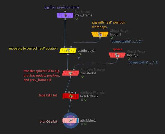
Like the earlier example, the trick is to merge the previous frame results with the 'live' geo from input1. Here I use an attrib copy to update P from input1 onto the previous frame geo, so the position is now correct, but the colour information will be the same faded result from the previous frame. Attrib transfer (and blur) as before, win.
Pop solver vs sop solver vs dops
It doesn't take a big leap of logic to realise that this a solver sop could be extended to a simple (or even a complex) particle system. Chain a vop network inside the solver to add noise, add a wrangle to check for collisions and so on. Ultimately, you can think of pops in this way; a glorified sop solver with nice gizmos for creating fields and forces.
In fact, this holds true for all the dop solvers, in a certain way. The core feature they all share is the ability to calculate a frame based on the result of another frame. Pops are a good way to get into sop solvers, and vice versa. It's all connected.
In fact, you might have noticed while working in a sop solver something odd; occasionally when diving in and out of the solver you'll end up in a weird in-between network. If you look at the network path you can see you're not just in a single subnet, but several levels down. Manually browse around in there, and the truth is revealed:
The sop solver is actually a dopnet in disguise! When you dive inside a sop solver, Houdini is doing some UI tricks to skip the subnet, and the dopnet in that, and an intermediate level below that, to take you directly to the innards of the solver. And keep in mind this works in both Escape and Master. That means....
Sop solver as cheapskate dynamics in Escape
Given the few examples outlined above, if you're on an Escape license (which lacks all the dynamics tools), you could go crazy and implement your own simulation framework. In theory all you need is access to the previous frame to do simulations. Of course you won't have access to pre-defined dynamics forces, or gizmos, or optimised workflows, or all the cool stuff a full Master license provides, but bah, where's the fun in using pre-packaged solutions?
Sop solver uses in dops
From what I understand, solver sops started as a way to access sops inside dops, before someone at sidefx hit upon the idea of using sops-inside-dops-inside-sops as a way to do all the time based effects we've discussed so far.
So why would you want to access sops within dops? Lots of reasons! For starters, constraints for rigid bodies and wires are represented as poly edges. Creating, modifying, deleting edges is easy in sops. Being able to access the previous and current frame is required to know when and where to create edges. Combine those two in a sop solver, you have a world of fun. I have an example of this at the end of the HoudiniDops page, where a sop solver is one of the inputs to a constraint relationship node. It uses a 'connected adjacent pieces' sop to build edges between any wire points that get too close, and those edges are converted into constraints.
Other uses are for splitting dynamics objects into smaller ones, or duplicating particles, or reading geo from sops using object merges, and using that to affect a simulation, or a myriad of other use cases.
They can also be used to modify attributes in ways similar to the growth/colour change examples. Eg, you could have an @active attribute grow throughout a sim using attribute transfers or wrangles, so that pieces of an RBD sim only turn active based on some other input. The advantage of doing it in a solver rather than other means is you can make it be a 'one-way' switch; ie once an attrib is turned active, you can design the sop solver in such a way that it won't turn off again (easy when you can compare previous frame to current frame), which can be tricky to do via other means.
When to use, when not to use
Once I 'got' solvers, I started applying them to every problem I had. I've seen other new users of Houdini do the same, its an easy trap to fall into. Often the logic can be easier to understand with a solver ('if the previous frame is x, then do y'), but be careful! Even though solvers tend to be fast, its still a simulation, meaning all the issues that come with a sim; you need to run the entire framerange, you might need pre-roll, and if the shot is 3000 frames long, and you need to look at frame 2940, well, you have to sim the previous 2939 frames to see it.
A co-worker gave some good advice to help break me from my solver addiction. He said 'Imagine you just had to brute force keyframe this problem... could you do it? If you can, maybe you don't need the solver sop.'. For example:
- Do you need to grow your colour based on nearby points, or could you just keyframe a ramp moving on the x-axis with some noise?
- Could you compare your points attributes against a certain @Frame or @Time, and trigger that way?
- Could you get away with just an attrib transfer, or some careful manipulation of noise?
- Does the behaviour roughly fall into a looping time pattern of a triangle/sawtooth/square/wave? If so, you can carve @Time in all sorts of ways in a wrangle to make it do cool things.
This falls into the larger 'simulation vs proceduralism' debate, which is always fun to argue. These days I tend to fall into the procedural camp, but its always good to know solvers are there if you need 'em.
Example: Transfer pop colour onto geometry
Download scene: pop_cd_solver_transfer.hipnc
Aka wetmaps, aka persistent impact, aka... lots of terms, its probably the main reason people use solver sops, very useful. If you've read all the previous bits this should be pretty simple. A grid is made black, and a pop sim is setup with coloured particles. Both are fed into a solver sop, and an attribtransfer sop is used to transfer Cd from the particles onto the grid. Because its within a solver, the effect is persistent, and builds up over time.
I've also included 2 other ways that give more control, one in vex, one in vops. Attribtransfer is actually doing quite a lot under the hood, so there's a little more stuff to recreating it in vex than you'd think. Here's the idea (remember, while I talk about 1 point on the grid, because this is vex it really means all points on the grid are doing this in parallel):
- Find the closest particles to the current grid point, store their id's in an array
- Loop through the particles found and:
- Get their position
- Get their colour
- Measure the distance from the particle to the grid point
- If its under a certain threshold:
- Add the particle colour to the current point colour
Like I said, more work. The advantage though is this gives you way more control. You can multiply the particle colour down by 0.1, so the colour builds up gradually, you can clamp the values so they never go above one, you can fade them over time by taking the final result and multiplying it by 0.9 each frame. Powerful stuff.
Example: 1960s style motion graphics
Download scene: solver_mograph_setup.hipnc
John Witney did beautiful animations in the 60s with early computer graphics; a lot of it was shapes under simple keyframed control, shot with multiple exposures and feedback loops to build complex motion graphics: https://www.youtube.com/watch?v=BzB31mD4NmA
That technique can be easily recreated with a solver. Setup a few transform nodes to spin and transform a shape, feed it to a solver that is set to both merge and transform the result, all sorts of trippy fun can be had. This is a time hole, you have been warned!
Example: slitscan

Download scene: slitscan.hipnc
More 60s inspiration! Been reading some interesting stuff on Roy Wiggins great website ( http://roy.red/ ), one of those was how to replicate the old Dr.Who time tunnel effect in webgl. I've been interested in this slitscan technique for a while, finally thought to implement it.
The idea is simple; setup a grid of points, texture it with some varying input (a spinning/sliding mandril in this case), and mask off a center section of it. In a solver, have each point look a short distance towards the center, and get colour from that location, blend it with its current colour. After the solver set the center to black, you have a time tunnel.
Shame you can't do a solver in cops though... RFE for the next version of houdini....
Example: Reaction diffusion
Download scene: reaction_diffusion_heightfield.hipnc
I've wanted to understand this effect for a while, but while there's been several examples floating around, I was determined to get it working myself. 3 years later, having tried it every 3 or 4 months, I finally got it. 😃
It all runs in a solver sop, as the current frame is always based on the previous frame. Reaction diffusion (RD for short) can be quite slow to progress, so I take advantage of a solver sop feature, substeps. By setting the sub-steps parameter to 20 on the top of the solver, that makes it run 20 times on each time step. It's not magically making it faster, but just saves the results of every 20 calculations to 1 frame, so you don't have to let the thing run for 7000 frames to start to see interesting things.
The RD equation is well explained on pages like this great one by Karl Sims, but I had a few things I wanted to get with my setup. It seemed like heightfields were the best solution for this, in that the core data type is a 2d volume, so its not wasting memory and time on connectivity information with edges and whatnot, and has less data requirements than just a grid of points (each 2d voxel just stores height, not a xyz position nor the potential to store more info). Plus heightfields have nice visualisation options, plus lots of nice ways to define patterns and shapes, plus the option to get a good performance boost with OpenCL if I'm ever brave enough to try that.
Anyway, the RD system requires 2 'chemicals', so I setup 2 heightfields, a and b. I then use a few methods to setup interesting initial states for the chemicals, the default is to flood chemical a with a value of 1.0, and chemical b with some pattern. The gif above uses a flattened pig projected onto the heightfield.
Inside the solver is a volume wrangle with the base equation. Getting the details right here is what took me so long, first in terms of how to read and process volume values (in the end its pretty straightforward vex, not sure why I couldn't get this working before), and secondly how to implement an interesting mathsy part of the RD equation.
In the wrangle I call these terms va and vb, which in the equation is the upside down triangle. This is the laplacian, which sounds fancy, but ultimately is a way to say 'calculate a value for a voxel based on the neighbouring voxels'. It's closely related to image processing, you might've seen convolution filter examples where if you sum up the neighbours to a pixel one way you get an edge detect, do it another way you get a sharpen, do it another way you get a blur. There's some good interactive examples of this you can play with here: http://setosa.io/ev/image-kernels/
Here I use the volume convolve sop to do this. From what I understand this particular arrangement (-1 in the middle, .5 for neighbours, 0.25 for nearest diagonals) calculates the difference of each voxel to its neighbours. This result (the lapacian of a and the laplacian of b) is then referenced in the main volume wrangle, as well as other key values from the original equation like f for a feed rate and k for a kill rate. You can look up the values on this table to get a sense of how f and k affect the final result:
http://mrob.com/pub/comp/xmorphia/
The wrangle looks like this:
vex
float da, db, f, k,dt, va, vb;
da = ch('da');
db = ch('db');
f = ch('f');
k = ch('k');
dt = ch('dt');
va = volumesample(1,'a',@P);
vb = volumesample(1,'b',@P);

@a += (da * va - @a*@b*@b + f*(1-@a)) *dt;
@b += (db * vb + @a*@b*@b - (k + f)*@b)* dt;
float da, db, f, k,dt, va, vb;
da = ch('da');
db = ch('db');
f = ch('f');
k = ch('k');
dt = ch('dt');
va = volumesample(1,'a',@P);
vb = volumesample(1,'b',@P);
@a += (da * va - @a*@b*@b + f*(1-@a)) *dt;
@b += (db * vb + @a*@b*@b - (k + f)*@b)* dt;The first chunk of lines are just to setup variables, and read the values from the volume convolve. The last 2 lines are pretty much reading the equation from the karl sims page.
Another key thing that tripped me up was misreading the lapacian bit. It's written as upside-down-triangle-squared, which I took to mean that I would replace that with va*va, and vb*vb. Took a long time to realise that no, I don't have to square the value, I just use it as-is. No wonder I flunked engineering maths. Ugh worse, I just looked at the wikipedia article, and there it is in the second sentence, saying it can be written like this or this or this. Sigh.
Why all this effort? Well, similar to the early back and forth with the differential curve growth thread on odforce, while it's fine to do the whole thing in vex and be a code rockstar, its not very modular or artistically tweakable. I feel that the combo here of heightfields, convolve sop, heightfield visualizer, is a pretty powerful combination. Changing patterns is easy, changing RD equation values is easy, changing the convolve operation is easy (most other implementations I've seen are pretty hard coded and brittle), this is ripe for experimenting and breaking in fun ways.
SDF growth
Download scene: sdf_advect_growth_v01.hip
This is totally a steal of Ian Farnsworth's amazing recursive growth blog post, I looked at his setup, then had a go at recreating it from scratch.
Tommy is converted to an sdf, and inside a solver a vdb analysis generates a gradient vel field which is perpendicular to the surface (you could think of it as generating N for the surface, in volume form). This is used to advect the SDF surface a small amount with a vdb advect sop. To get the interesting lumps and stuff another analysis sop is used to measure curvature. Flattish areas get a low value, curvy creased areas get a high value. The vel field is multiplied by the inverse of this curvature, so that creases are mostly unaffected, while smooth bits get inflated.
The fun thing about doing this in a solver is adding mini or macro disturbances to the vel field before it advects the surface. Little bits of micro noise to encourage little polyp growths, large scale noise to globally warp into more interesting shapes, or addition twist or localisation forces.
Image feedback with heightfields
Download hip: sops_hf_feedback.hip
More of the same, kind of works, kind of effort. To work with images you need to track the r g b channels yourself, which is dull. Cops used to have a feedback node but it was removed. Doh.
This has some token efforts to speed it up (a compile sop that probably does nothing, convert to polysoup rather than polys, other red herrings), but ultimately it's a lot of effort for not much gain. Just use regular geo like the slitscan/1960s examples earlier.
Cube slice
Download hip: cubeslicesolver.hip
I saw this lovely tweet from Frederik Vanhoutte aka @wblut, and immediately wondered how I'd recreate it in Houdini. I'd done similar work before using compiled recursive clips in a for loop, the core idea is pretty much identical, just running in a solver instead.
Every second the cube is clipped, and one half of the clipped geo is rotated. There's some stuff to choose a random clip vector, and make sure that its passed down to a wrangle to rotate around the same vector. The only other bit of trickery is a channel ramp to control the easing and fake spring 'ca-chunk' at the end of the rotation. The polyfill to cap the ends of the clip gets easily confused which is a little disappointing, but happy to park it here for now. Should be ripe for building on and getting cooler motion should anyone be keen to try.
Someone asked why I used a clip sop rather than booleans. The reason is "I didn't think of it". Had a go, sorta works, sort of still has issues. Have a look:
Download hip: cubeslicesolver_booleans.hip
Non solver sop solvers
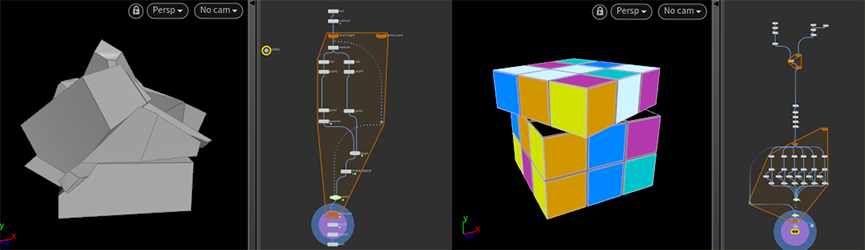
Special guest content from Luke Van, thanks!
Download hip:slicer.hip
Download hip: rubiksCube.hip
My general take on solvers is 'if a system is going towards unbounded complexity, a solver sop is the way to go'. The clipping cube example above and the rubiks cube example elsewhere I felt were ideal examples of this.
Well, along comes Luke to prove me wrong. He's worked out a way to use For Loops to get the same effect, but its deterministic. No caching of frames required, just jump to a time offset, bam, result is calculated.
Luke writes:
A fetch feedback loop is essentially copying the node tree inside of it a bunch of times, and wiring them in line, and having a useful attribute of which copy you are on. With that considered, everything in the loop is fairly self explanatory, and then the transform sop is where the so called 'magic' happens. If you think about isolating each loop into its animation, you need a 90 degree rotation over a period of time, lets say 25 frames in this case.
This can be easily done with
fit($FF, 0, 25, 0, 90)
If you put this in the loop, all of the transforms are happening at once, so I used the iteration to offset it:
fit($FF, iteration*25, iteration*25+25, 0, 90)
The bit with iteration*25+25 is basically finding the end point of the animation, but first finding the start point (iteration 25) and then adding the animation duration.
Now that this works, we can go a step further and throw that whole thing into an ease with
`chramp("ease",fit($FF, 0, 25, 0, 1),0)90`
The fit is changed to sample between 0 and 1 and multiplied by 90 afterwards, rather than just 0 and 90. Once you sub out the pseudocode for the correct references to the meta import node of the loop, you're all set.
Thanks again Luke!
Other examples
A quick search for 'solver houdini' found these great examples:
- recursive growth: https://vimeo.com/154251482
- simple crowd: https://vimeo.com/143691632
- furl/unfurl: https://vimeo.com/111728110
- gradual build towards chaos, eg messing up a rubiks cube: https://www.youtube.com/watch?v=DWjfprJlH0s
- steering behaviours (similar concepts to crowd): https://vimeo.com/142783022
- tile flipping: https://vimeo.com/111246905
As a final bit of homework, which of those could also be achieved procedurally, and thus not require simulation?