Volumes ​

Volumes are primitives ​

Confused me slightly at first, so worth mentioning; A volume is a primitive, the same way that a point is a primitive, or a primitive sphere is a primitive. This means that unlike a polygon mesh for example, there's no drilling down to its sub-components; you can't open the geometry spreadsheet to see values in the individual voxels.

There are other tools to help you see whats going on within a volume (volume slice sop, volume visualisation sop, volume trails sop etc), but ultimately, if you merge a 400x400x400 voxel volume with a primitive sphere, if you inspect the merge it will show that you have 2 primitives; a volume and a sphere.

Houdini supports 2 volume types, its own volume format, and VDB. These are treated as primitives like polys or nurbs, if you middle click and hold on a node, you'll see it say '1 VDB' or '1 Volume' or similar.

VDB? ​

The most simple way to describe it is as Alembic, for volumes. It's an open source, standardised format so you could export a VDB from Houdini, load it into maya, and render in Vray. It has several companies helping drive it (Dreamworks, Double Negative, SideFx being the most notable), and is generally a good thing.

It's more than Alembic though, in that Alembic is mainly a file format, and a handful of example tools to manipulate and view Alembic files. The VDB toolkit is both a way to store a volume, and a large suite of algorithms to manipulate volumes.

One of VDB's most interesting qualities is that it doesn't waste storage space on empty voxels. VDB's can be substantially smaller on disk compared to other formats.

The VDB storage format is exposed in Houdini as a primitive (a 'VDB primitive' funnily enough), and the manipulation tools are exposed as sops, mostly with the VDB prefix or suffix.

The name VDB as stated in the original paper comes from "...Volumetric, Dynamic grid that shares several characteristics with B+ trees.".

Further reading: http://www.openvdb.org/about/

VDB interactive tutorial ​

A fantastic walk-through of VDB features is also available from the openvdb website. It's a single houdini file that is like an interactive book on VDB; its broken into chapters, lots of sticky notes, I'm surprised I only found this recently. Many thanks to the person on odforce who pointed it out! If you want to use VDB like a boss, download it RIGHT NOW.

http://www.openvdb.org/download/

VDB vs Houdini volumes ​

Houdini's own volume format had been around for a while before VDB arrived, so there's a large amount of nodes in there for working with them (you can see this in sops by typing 'volume' in the tab menu). VDB has its own collection of nodes (either prefixed or suffixed with VDB).

VDBs can be substantially smaller than native Houdini volumes (savings of 50% are common), and often the VDB sops are faster and have more interesting features than the native Houdini volume sops.

There's a .vdb file format (which you'd use to export to other apps), but you don't need to write out a .vdb file to get the space savings, just having a VDB primitive in Houdini is enough. A Houdini volume primitive can be converted to a VDB primitive at any time, just put down a convertvdb node, set its mode to VDB. If you middle click on the node, you'll see the Volume primitive has been replaced with VDB. You can now cache this out to .bgeo like any other piece of Houdini geo, but it'll be much smaller than if you didn't convert.

What's nice is that a lot of the core Houdini volume tools have been updated to work with VDB primitives too. Volume VOPS and Volume Wrangles for example both work with VDB. This means its pretty safe to use VDB at all times, as you can easily convert a VDB temporarily to a native volume if required, and then convert back again.

Further reading: http://www.sidefx.com/docs/houdini15.0/model/volumes

Scalar and vector volumes ​

A volume used to represent a cloud for example only needs to store a single value per voxel, density. If density is 0 the voxel it is completely transparent, if density is at 1 the voxel is opaque. The cloud sop for example uses noise functions under the hood to sculpt density into pleasing cloud shapes.

If you wanted to store colour that varies through the cloud, then you need to store the red/green/blue components. This means you require a vector volume (or vector field, you'll find the docs and forums refer to volumes as fields a lot), to store this information.

A more common use of vector fields is for velocity. A convention in Houdini is that a velocity volume is named 'vel'. Each voxel in the volume stores a direction. A pyro solver will use this velocity field to transfer density around, giving the impression of movement. Other properties of pyro sims is to modify the velocity field itself, so you might get a mushroom cloud that rolls upwards, or noise that swirls the density around.

Something to note is how native Houdini vector volumes and vdb vector volumes differ. Internally Houdini doesn't really have a vector volume format, but it creates 3 scalar volumes, and knows to treat them as a single entity. A standard smoke setup that uses density and vel will have 4 volume primitives; density, vel.x, vel.y, vel.z.

VDB does support vector volumes, so the same smoke setup will be 2 vdb primitives, density and vel.

Note here that its almost the reverse of how you work with standard geometry and attributes;

• A grid is a single piece of geometry, but each point on the grid might have many attributes (N, Cd, id, foo, myattr etc.)
• A volume primitive can only contain a single attribute, so instead you make multiple volumes, each one storing a single attribute (density, vel, fuel etc).

Some tools in Houdini know this, and know how to wire all the volumes up and treat them as a single entity. Others don't though, and you need to explicitly tell a pyro solver, for example, to also modify the Cd field along with density and velocity (an example of this is further down).

Most of the time you're dealing with the default fields Houdini expects, so this hand-wiring of fields doesn't happen often in practice.

SDF ​

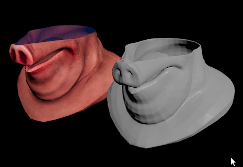
A volume (or vdb) can represent an amorphous shape like fog or fire, or it can represent a solid surface. When doing the latter, each voxel stores the distance to the closest point on the surface, and if its on the inside or outside of that surface. Because these values can be fractions (eg 1.42 units from the surface rather than just 1), they can give a pretty good approximation of the input geometry. To tell if a voxel is on the inside or outside of the surface, it becomes positive or negative; positive is outside, negative is inside. If you visualise it, it would look like a gradient that is 0 on the silhouette of the shape, and a smooth gradient that extends inside and outside the shape. This volume is called a Signed Distance Field, or SDF.

Positive values are red to yellow, negative values are dark to light blue.

This can be handy for many things. If you have a robust way to generate a SDF (which of course we do in Houdini), it's a great way to generate collision geometry for simulations. Particles or RBD objects can very quickly sample the SDF, if their sign is negative, they're inside the shape. They can then measure the gradient of the SDF, and determine exactly how far and how much to be pushed to stop intersecting.

If you take the SDF and convert it back to polys, you get an evenly meshed, watertight surface. You can smoothly expand or dilate the surface, you can combine SDFs and get very clean booleans, they're handy in lots of situations.

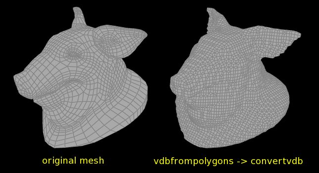Houdini gives you 2 ways to generate an SDF from poly geo; the native Houdini way ( IsoOffset SOP in SDF volume mode), and the VDB way ( VDB-from-polygons sop). My 30 second tests imply VDB is much faster for more detailed geometry.

Houdini visualises SDF volumes with a sprite per-voxel where the SDF field is 0. It looks like it uses the SDF gradient to derive a normal for the sprites, so they respond to lighting.

Viewing volume data ​

Download scene: vis_volume.hip

Because a volume or vdb is treated as its own primitive type, the voxel data can't be inspected from the geometry spreadsheet as you'd initially expect. If you try, all you'll see is a primitive number for each volume.

Instead, you're supposed to use the visualise tools within the viewport. A Volume slice lets you see a 2d slice of voxel data mapped into a colour ramp, a volume trails node lets you follow lines of direction within a volume, say graident, through the volume.

The example hip is an example of the two different ways of working with volumes; it calculates the gradient in 2 ways, one with a vex 'volumegradient' call, the other with the 'VDB analysis' sop. The VDB nodes are presented a little differently than regular Houdini nodes, but are very powerful and very fast.

Volumes, SDFs, Trails ​

Download scene: volume_trails_V01.hip

Saw an interesting vimeo tutorial on generating swirly lines ( https://vimeo.com/134057856 ), and an odforce post asking how to generate tracer lines from noise ( http://forums.odforce.net/topic/23535-noise-how-to-convert-into-line/ ), this is my attempt to combine the two. The volume trail sop is used to visualise fields in volumes, but you can use it for your own purposes if you get volumes setup the right way.

Here, the idea is to take a shape and create an SDF, or Signed Distance Field out of it. This is a volume where each voxel stores the distance to the closest point on the surface. Voxels on the surface have value 0, voxels outside the surface have positive values, voxels inside the surface have negative values. This makes them very handy for checking collisions, among other things (here's a nice shadertoy demo to visualise SDFs in 2d: https://www.shadertoy.com/view/ltBGzK )

I then take another volume, where each voxel can store a vector value, called 'vel' (the houdini standard for storing velocity in volumes). I then clip the vel field using the SDF, so only voxels within 0.1 of the surface remain, the rest are clipped.

I then run that volume through curl noise, so the vel field now has groovy lumpy swirls through it. Feeding that to a volume trails sop generates the sweet lines.

While this sort-of follows the pig surface, the lines tend to wobble above and below the surface quite a bit. To make them stick directly on, I just ray the curves onto a slightly fatter copy of the pig (to avoid clippy intersection issues).

There's probably a way to generate the curl noise directly from the SDF, so that the resulting lines stick dead on the surface. A ray is quick n lazy tho. 😃

Volume magnetic lines ​

Download scene: magnetic_lines_vdb.hipnc

Found this post ( http://pepefx.blogspot.com.au/2015/08/how-to-create-magnetic-vector-field-in.html ) explaining how to setup magnetic lines. Tried to follow it once when very tired, then tried it again a month later without looking at his notes to see if I could get a similar effect, and without using his clever vex.

Two things that might be interesting in this setup:

• Creating vdbs from polys, specifically creating density and vel vdb's simultaneously from the one poly. The vdb-from-polygons sop has a multilister similar to creating aovs/image planes on a rop. Click to add a new one, tell it what attribute is the source (eg, v for velocity), and what kind of vdb it will map to (vector).
• Combining vdb's. I setup a positive and negative vdb, then combine them with the 'add' mode. It just occurred to me I could have merged the poly shapes first, then made the vdb in one step, which would be much more efficient. Still, handy learning exercise eh?

The end result I'm sure is a scientific abomination, but looks pretty. To be honest I was sure the setup wouldn't work; just creating a negative and positive velocity field seemed too simple for the volume trails to do its thing, but here it is, working. The lines and colours are my usual abuse of volume trails and point wrangles.

Swirly lines, or worms with volumes and curl noise ​

Download scene: vol_worms_curlnoise.hipnc

Another attempt at the swirly lines thing, but I think much more effective. I'd seen Raph's very cool experiment on vimeo, and was curious about how it was achieved. Naturally being too proud to ask him even though he sits 2 metres away from me, I'd been stewing on it for a while.

My experiments in pyro got me familiar with volumes and creating velocity fields, and the volume trail sop kept giving cool results. Was using curl noise in a volume vop when I noticed the input for a sdf. Started playing with it, to my surprise it does exactly the effect I was after, and the help docs confirmed it; like putting rocks in a stream, it forces the curl noise to flow around the sdf's you give it.

As such, the workflow is this:

1. Take a shape (the trusty pig in this case)
2. Get its bounds, make a vel fog vdb from it
3. Also make a SDF of the pig
4. In a volume vop, use curl noise, attach the SDF to the input of the curl noise to 'disturb it', adjust sliders to taste
5. Test the vdb for negative values (ie, inside the pig shape), make those values 1, outside values 0
6. Multiply the curl noise against this to set all vel outside the pig to 0. Now the curl noise flows along the surface and inside the pig volume
7. Scatter points on the pig surface, volume trail sop to generate cool lines
8. Either use @width to render the curves directly or polywire sop to get poly tubes

Curves with @width are more efficient of course, but there's a bug with them and opengl that causes odd spikes and pops, so I need to fall back to polywire for my flipbook captures. The dancing lines are from adding time to the inputs of the curl noise.

Here's the same effect applied to the squab, with the addition of colour being driven by the SDF values in turn driving a ramp; values near the surface are white, then red, then pink, then blue. Pleasingly gross.

Download scene: vol_worms_curlnoise_v02.hipnc

Convert geometry to velocity volumes efficiently ​

A 'vdb from polygons' node works great for converting meshes into sdf or fog, and can create a velocity field too if you have @v on your mesh.

Eg, I have a pig, give it point normals, create a swirled @v in a wrangle with @v = cross(@N,{0,1,0}); then use 'vdb from polygons' to make a density field, and additionally create a @vel field from @v. (I also append a scatter and volume trail to visualise the swirly field):

If you don't have a watertight mesh though, it confuses the vdb convert sop quite badly, so either require very dense sampling settings, or you have to create manifold geo with extrudes and whatnot, which may not be possible.

Here I swap the pig for a curve that has normals and velocity. The vdb from polys node can't make a density field, so the whole thing breaks:

What we really need here is a to be able to make a generic fog of density, and then do an attribute transfer of @v from the curve to @vel of the volume. There's a few nodes to do this (volume from attribute, velocity volume, volume from curve etc), but unfortunately all seem to not work with vdb, only regular houdini volumes. That then means you'd convert, do the thing, convert back, which is wasteful.

A better way is to use a volume wrangle:

Here's what's going on in that gif:

1. We need a generic box of density to start with, so I use a bounds sop from the pig, and feed that box to the vdb from polys
2. The vdb node gets a little confused, as it was creating vel from @v, which the box doesn't have. A quick reset to nothing, then P, clears its head. So for now @vel is actually storing @P, but this is just a placeholder
3. A volume wrangle is appended after the vdb node, all it does is 2 things:
   1. int pt = nearpoint(1,@P); --- for each voxel, find the nearest point on the curve, get its @ptnum, store it as pt
   2. v@vel = point(1,'v', pt); --- lookup point pt on the curve, read its @v, store it in the current voxel as @vel
4. Wire this into the volume trail to see the result.

Note that I use v@vel rather than just @vel; I was surprised to find that @vel isn't one of the 'special' wrangle attributes that automatically knows what type it should be. If you forget, it gets treated as a float, which caused me much confusion for a while.

Here's the scene: volume_vel_from_geo_curve.hipnc

Thanks to Luke Gravett for showing me this little trick.

Volume displacement ​

Download scene: volume_disp_example.hip

Once again, had built this up as something really complicated in my head, when in fact its very easy. Generally speaking volumes look better when you use smaller voxels, but of course this comes at the cost of disk space, memory, render times. I was aware that Houdini and mantra supported volume displacement, but I think whatever tutorial I looked at made it all seem very complicated.

Some prompting from Patreon supporter Isaac Katz made me go do some research, and it led me to a simple example by Marc Picco on the odforce forums. All you do is setup the shader as you would for regular polygon displacement, so take P, add some noise, feed to a displacement output.

The gif above shows how effective this can be; the starting res for the volume pig is very low (25x27x29, just enough to capture the basic pig shape). By displacing at render-time, this gets pixel-level detail (or even sub pixel assuming the noise driving the displacement is fine enough, and you zoom in close enough), and the render times stay pretty reasonable.

This shows the extra nodes I added to the 'basic smoke' shader from the material palette, the only confusing bit was how to create the displacement node; all it is is an output node, with the type changed to 'displacement'.

Volume deform ​

Download scene: volume_deform_simple.hip

Deforming volumes seems like it should be simple, then you try it and realise it's not. There's frustratingly cool in-house tools like REVES at Pixar that seem to handle it effortlessly, but what do the rest of us do?

Well, there's the right ways to do this (like the [https://www.orbolt.com/asset/StianHalvorsen::Volume_Lattice Volume Lattice asset on Orbolt], or this example by Juraj Tomori ), both of which do it as a direct conversion with volumes, and there's this slightly hacky way. After reading a hint on how to do this on a vimeo post that I've lost, and a hint from a co-worker, this isn't too bad, and its fairly fast on reasonably high res volumes.

There's 2 parts to this, one is to convert the volume to points using a vdb visualizer, the other is to convert back to volume using volume_from_attribute.

The vdb visualizer can generate an exact conversion from volume to points. If you change its mode to only operate on active voxels, and export points with values, then that's what you get; a point for every voxel, with its density stored as @vdb_float.

Now that its points, you can apply deformation as you see fit, here I've just used a lattice.

To convert back to a volume, I use a bounds sop to get the bounding box of the deformed points, then vdb_from_polygons to get a fog vdb, and a convert vdb to change it to a houdini volume (my quick tests imply it's faster to do this than to use an isooffset sop). Now that there's a volume, I create a volume_from_attribute sop, connect the new volume to the first input, and the points to the second.

This does as it says, it reads the point attribute you specify, and copies it to the volume. By tweaking the settings on this node, and the resolution of the vdb_from_polygons sop, you can get a good compromise between detail and processing speed. Note that it doesn't support VDB, hence the conversion to a standard Houdini volume.

I still want REVES though.

Volume deform v2 ​

Download hip: vdb_deform_v02.hip

Revisited this after a question on patreon/discord. Essentially the same technique as before, but using the Volume Rasterize Attribute node to convert points to VDB. Even though its based on VDB under the hood, its substantially faster to process than vbd from particles or vdb fluid surface.

Here I take a run cycle, freeze a frame, scatter points, rasterize into a volume. I then use a cloud sop to cloud it up (and use the offset controls to animate the clouds moving), then vdb viz tree to get points, point deform by the original animation, and vdb rasterize attributes again.

Another bonus of using rasterize attributes is the good support for if the deformation gets too extreme or fast. If you have @v you can streak the volume with motion blur, if the points get too far apart and dotty, there's some controls built in to blur the result and hide the artifacts.

Still not quite REVES, but not bad.

VDB combine ​

Download hip: vdb_combine_2_methods.hipnc

I need to do this every few months, forget, swear, fumble around until I get it to work again. Thanks to sexyman Jake Rice, I realised my previous attempts were ovelry complicated, and combining vdb's is pretty easy.

Feed all your vdb's into a merge, connect the merge into the first input of a VDB Combine. Set collation to 'Flatten All A', and operation to 'Maximum'. The resample parameter lets you determine how the voxel size is chosen, in this case the options that make the most sense are 'lower-res to match higher-res' or vice versa.

If you want absolute control over the resampling, then make a solo vdb node, name it density, set the voxel size. Connect that to the first input of a vdb combine, run your other vdbs to a merge sop, and that into the second input.

In this case choose Collation to be 'Flatten All B into First A', Operation 'Maximum', and Resample 'B to Match A'.

Cloud light ​

Download hip: volume_cloudlight3.hipnc

The cloud light sop takes a volume and some points. It treats the points as lights and calculates an emission volume, which you can run through a ramp to get faked volumetric lighting. It's a bit fiddly to control, but you can get some pretty cool effects cheaply, meaning you might be able to avoid expensive volume pathtracing in your render.

SDF from open shapes ​

Download hip: sdf_from_open_shape.hipnc

Great tip from Kiran Irugalbandara!

SDF's are handy for collision geometry and whatnot,but can be annoying to deal with if you don't have watertight shapes. Sometimes you can get lucky with generating caps, or go brute force, scatter millions of points and treat it like a flip meshing operation, but neither felt like an elegant solution.

Kiran has the elegant solution. SDFs by default expect a watertight mesh so it can set the sign for being inside the mesh or outside. But you have the option to make it unsigned (UDF? USDF? Hmm). From that you can convert it into a signed distance field again with the convert vdb sop, and from that into polys once more if you need it, getting you your watertight mesh.

Thanks for sharing this trick Kiran!

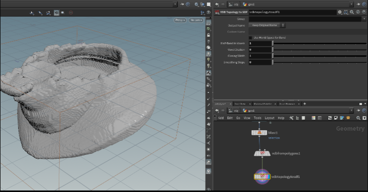
TIME PASSES

Well not that much time. Shortly after posting this, Paul Ambrosiussen said there's an easier way. Do your regular vdb from polygons, see the janky result, and then append a VDB Topology to SDF. Boom, fixed.

Nice one Paul!

Jet exhaust or shock diamonds ​

Download hip: jet_exhaust_diamonds_v02.hip

Volume rasterize attributes is a very fast way to convert points to volumes. As such you can model shapes with points, getting attributes as you like, and convert to volumes at the last minute. This setup does that, and uses temperature values to drive the blue and red regions. It's highly controllable and requires no simulation, which is always a nice bonus.

I recorded a 60 second walkthrough of this setup for the 30 second quicktips colletion (I can't count to 30, sue me): https://www.youtube.com/watch?v=b9ctURcZyLc

Further learning ​

There's a long form tutorial on Smoke and Pyro, covers a lot of similar ground to this page, but explained in more of a linear fashion, and goes through the steps of building a smoke setup without using the shelf tools, I've tried to construct it as a clean standalone tutorial for anyone getting into pyro and smoke for the first time. You'll find it here: Smoke_and_Pyro.