Appearance
Vex Section 3
xyzdist to get info about the closest prim to a position

Download scene: Download file: xyzdist_example.hipnc
If you've used a ray sop, this is a similar thing. At its simplest, give it a position, it will tell you the distance to the closest primitive. More usefully, it can also tell you the primnum of that primitive, and the closest uv on that prim to your position. With this info you can then work out the position on the prim.
Like the matrix rotate() function, primnum and uv are set via pointers, so you create the variables you want first, then call them within the function:
vex
float distance;
int myprim;
vector myuv;
distance = xyzdist(1,@P, myprim, myuv);
float distance;
int myprim;
vector myuv;
distance = xyzdist(1,@P, myprim, myuv);To get the exact position of that uv on that prim, and the colour of the prim:
vex
vector mypos = primuv(1,'P', myprim ,myuv);
@Cd = prim(1,'Cd', myprim);
vector mypos = primuv(1,'P', myprim ,myuv);
@Cd = prim(1,'Cd', myprim);The above contrived gif shows all this in action. A point is orbiting the multicolour pig. xyzdist finds the distance, primnum, uv of the closest prim, a point is made at that location, its colour is set from the closest prim, a red line is drawn from the orbiting point to the new point, and finally a wireframe sphere is generated on the new point, its colour also matches the prim its currently on, and its radius is set from the distance returned from xyzdist, so it alwasy just touches the orbiting point.
Rubiks cube
Download scene: Download file: rubiks_cube.hipnc
As per usual I worked this out a while ago, forgot, took a few stabs to remember how I did it, fairly sure this method is cleaner than the original. Much thanks to Aeoll from the Discord forums for helping with the last bit I was missing.
This is a 3x3 box of points, with cubes copy sop'd to each point. This setup requires 2 things to start with, a random x/y/z axis to turn, and to select a slice on that axis to turn.
There's probably lots of very clever super compact ways to choose a random axis, I've gone something fairly lowbrow. Assume we have an integer 'randaxis' that can be 0 1 or 2, and a vector 'axis':
vex
if (randaxis==0) axis = {1,0,0};
if (randaxis==1) axis = {0,1,0};
if (randaxis==2) axis = {0,0,1};
if (randaxis==0) axis = {1,0,0};
if (randaxis==1) axis = {0,1,0};
if (randaxis==2) axis = {0,0,1};To generate randaxis, lets say we want it to randomly generate 0 1 or 2 every second. To do that we'll obviously need to use @Time as an input. To make time be stepped we can use floor(@Time). Feed that to rand to generate a random number between 0 and 1, multiply by 3 to get it between 0 and 2.999, and finally convert to an int to make it be only 0 1 or 2:
vex
int randaxis = int(rand(floor(@Time))*3);int randaxis = int(rand(floor(@Time))*3);So lets say we've randomly chosen the x-axis, {1,0,0}. Now we need to choose the left, middle or right slice to rotate. The cube is 1 unit wide, meaning that we can say for certain the left points have @P.x as -0.5, the middle as 0, right as 0.5. The same will be true for @P.y when choosing a slice on the y axis, and @P.z on the z axis. As such, we'll setup a float 'slice' to be randomly -0.5, 0, or 0.5 and use it later (randslice is generated in a similar way to randaxis):
vex
if (randslice==0) slice = -0.5;
if (randslice==1) slice =  0;
if (randslice==2) slice =  0.5;
if (randslice==0) slice = -0.5;
if (randslice==1) slice = 0;
if (randslice==2) slice = 0.5;Now we have an axis and a slice, how do we use this? We need to construct a test for every point against axis and slice, and if they pass, do stuff. Here's the test I use:
vex
if (sum(@P*axis)==slice)if (sum(@P*axis)==slice)Sum(vector) returns the total of the vector components, so sum( {1,2,3} ) returns 6 (ie, 1+2+3). For the top front right corner of our cube, ie {0.5,0.5,0.5} we'd get 1.5.
But here we first multiply @P by 'axis'. Lets see what that does to a few different points. If axis = {1,0,0}, ie, the x axis:
   {0.5,0.5,0.5} * {1,0,0} = {0.5,0,0}
   {-0.5,0,-0.5} * {1,0,0} = {-0.5,0,0}
   {0,0,0} * {1,0,0} = {0,0,0}
{0.5,0.5,0.5} * {1,0,0} = {0.5,0,0}
{-0.5,0,-0.5} * {1,0,0} = {-0.5,0,0}
{0,0,0} * {1,0,0} = {0,0,0}Ie, it has the effect of cancelling the y and components. Running sum() on those results above returns 0.5, -0.5, 0. In other words, we've extracted the x component from the vector as a float.
The next part of the test checks compares that result to the 'slice' var. Lets say slice is 0.5, how do those results compare?
   0.5 == 0.5, pass
   -0.5 != 0.5, fail
   0 != 0.5, fail
0.5 == 0.5, pass
-0.5 != 0.5, fail
0 != 0.5, failSo here we've said only points that have their @P.x match the slice we're interested in (0.5) pass, all other points fail.
Why this trickery? Well, we could do a big multi-level if statement that says if x-axis do this, else if y-axis do this, else if z-axis do this, then if slice1 do this etc... That gets very unwieldy and prone to errors. Here we've exploited some properties of how vectors multiply together to get a much cleaner test.
From here it's plain sailing. We know the axis to rotate around, so we do the usual matrix rotate dance, and update @P and @orient:
vex
matrix3 m = ident();
float angle = $PI/2*@Time%1;
rotate(m, angle, axis);
@P *= m;
@orient = quaternion(m);
matrix3 m = ident();
float angle = $PI/2*@Time%1;
rotate(m, angle, axis);
@P *= m;
@orient = quaternion(m);If we didn't have colours on the cubes, or motion blur, we could leave this in a normal wrangle and call it done. As soon as you add colours, you get the result on the left in the gif; each second the cube resets, it never shuffles. This is a good example of proceduralism vs simulation; the gradual descent into an ever more mixed chaotic state would be difficult to maintain procedurally, as you'd need to record ahead of time the entire sequence of moves, and track them all, and apply them at every time step. I don't think its impossible, but not easy.
Instead we can do what happens in the right cube using a solver. Rather than set explicit rotations, we set a small delta of rotation, and accumulate it each frame. This means changing 'angle' in the above code block; rather than being driven by @Time%1 so it cycles, it uses @TimeInc (ie, 1/24th of a second in standard Houdini):
vex
//angle = $PI/2*@Time%1;
angle = $PI/2*@TimeInc;
//angle = $PI/2*@Time%1;
angle = $PI/2*@TimeInc;Well, almost. In practice the final rotation isn't quite mathematically perfect, so rather than the pieces snapping into -0.5, 0 or 0.5, it goes to 0.000000001 or 0.49999999999. This is enough to throw the test, so pieces start to break. Aeoll from Discord was kind enough to show how to get around it, namely by modifying the test to allow a little bit of slack:
vex
if (abs(sum(@P*axis) - slice) <= 0.001) {if (abs(sum(@P*axis) - slice) <= 0.001) {There's more minor changes in the hip file (everything is driven by a time var 't' rather than @Time so I can speed things up or slow it down, and a few other things), but that's the core of the effect.
Sliding puzzle
Download scene: Download file: slide_puzzle.hip
Feels like there's a more elegant way to do this, but was a quick attempt while waiting for renders, leaving it here as a taunt to myself to improve it...
This uses some vex in a solver sop, the idea is that one piece (piece 0) at the start of each time interval looks at its neighbours, and chooses one at random. For the rest of the time interval it interpolates from its current position to the target neighbour, while making the neighbour do the reverse. After the solver I hide that piece, so it looks like the rest of the pieces are shuffling into the spare slot.
The lack of elegance in the solution comes down to my usual problem with solvers; I'm always off-by-1, or the calculations are off by a tiny bit within my loop, so that pieces get stuck, or double up, or do other silly things. Here I had to double check that the pieces don't inadvertently set their current and target positions to the same value, that the rest positions are nice and clean, and a few other fiddly things that I wouldn't think I need to do. One day I'll have an amazing mental library of slick elegant algorithms, but not today... not today...
Vex vs Vops
If you've read this far, you might be thinking 'Wow, I'll never use vops again!', or 'Ew, vex looks horrible! I guess I'll stay with vops!'.
You don't have to choose one over the other! Remember, vops generate vex, so it makes sense that they can happily co-exist. Within vops, Houdini provides two handy nodes, 'inline code' and 'snippet'. Both let you write vex within vops, and wire attributes in and out of them just as you would with regular vop nodes. There's some subtle differences compared to wrangles, but the point is that you can use vops when that's a better fit (manipulating procedural textures like noise is much easier in vops), and swap to vex when it's the better option, eg if/for/while loops.
Vex snippet cheat sheet
I don't use these enough, so always forget the right way to use em.
Connect all your input attributes, refer to them directly without any $ or @ prefixes. Every input will have a correspoinding outname output, just connect the output you want to the next vop.
If you need a new placeholder variable, best to create a constant of the type you need, name it appropriately, set its value within the snippet, then use its out_name to feed to the rest of your network.
Eg, here I have a string being generated from the renderstate vop, and I want to make a random float from that. I know there's a vex command, random_shash() to do exactly that. So I make a snippet, connect the renderstate, create a float constant called 'myrand', wire that in, and in the snippet refer to the input names directly. I then take the output value of myrand, and connect that to my network. (I found for some reason that just the object_name by itself always returns the same result, so I append an underscore, that makes it behave. Weird.)
If the default names from your input nodes aren't to your liking, you can drop a null in-between to give you nicer names. Remember, a null can handle multiple attributes at once, handy:
You can do all that directly on the snippet node (that's what the 'variable name 1, variable name 2' things are for), but I find it easier to pre-filter the names before wiring to the snippet.
Vex includes

You can create libraries of functions in external files, and pull them in as you'd do in C.
To start with, make a vex/includes folder under your houdini preferences folder. So in my case on windows, that's in my documents folder, houdini16.0/vex/include. In there I've made a text file, foo.h, and defined a simple function:
vex
function float addfoo(float a; float b)
{
    float result = a + b;
    return result;
}
function float addfoo(float a; float b)
{
float result = a + b;
return result;
}The specifics there are that I've defined a function that takes 2 float variables, and returns a float.
In houdini I made a wrangle, and that calls the above function:
vex
#include "foo.h"
@a = addfoo(3,4);
#include "foo.h"
@a = addfoo(3,4);A mild issue I ran into was updating foo.h, but houdini wouldn't detect the change. I figured toggling the bypass flag would be enough, but no. Turns out houdini only triggers a vex recompile if it detects a code change to your wrangle. Luckily this can be as simple as adding a space or a carriage return, then when you hit ctrl-enter, you'll get the update.
If you want to put your includes somewhere else, you can append to the system variable HOUDINI_VEX_PATH.
Spherical and linear gradients
Download scene: Download file: gradient_spherical_vs_linear.hip
Interesting question from a Patreon supporter. You have 2 locations, and want to use these to define a gradient on some geo. When i asked if he wanted a spherical gradient (so point 1 is the center, and point 2 defines a radius), or if he wanted a linear gradient (so p1 defines the start, p2 defines the end), he said 'yes' to both.
A spherical gradient is easy enough, the core is measuring the distance from your geometry to a point, p1 in this case. There's a built in vex function for that, so we'll use that. The result of that visually isn't often what you want, as it'll be 0 at the center (cos the distance from your sphere center to those points is 0), and gradually increase the further away the geometry is.
Instead you want to reverse that, so that its 1 in the middle, and goes to 0 at the radius you specify. How to do that? Well, easy enough to make the colour be 1, and then subtract the distance result. But to make sure the distance is black at the exact radius we want, we can divide the distance by the radius (which is the distance between p1 and p2):
vex
vector p1 = point(1,'P',0);
vector p2 = point(1,'P',1);

float r = distance(p1,p2);
@Cd = (r-distance(@P, p1))/r;
vector p1 = point(1,'P',0);
vector p2 = point(1,'P',1);
float r = distance(p1,p2);
@Cd = (r-distance(@P, p1))/r;The linear gradient question was more interesting. My initial tack was to to set p1 as the origin (so a way to do that is to subtract @P - p1), then calculate a quaternion that'll rotate the positions to align with the p1->p2 vector. It works, but its overly complicated. Here's that code:
vex
vector p1 = point(1,'P',0);
vector p2 = point(2,'P',0);
vector xaxis = {1,0,0};
vector aim = normalize(p2-p1);
float d = distance(p1,p2);
@Cd = @P-p1; // set origin to sit on p1

vector4 q = dihedral(aim,xaxis);
@Cd = qrotate(q, @Cd);
@Cd = @Cd.x / d; // normalize
vector p1 = point(1,'P',0);
vector p2 = point(2,'P',0);
vector xaxis = {1,0,0};
vector aim = normalize(p2-p1);
float d = distance(p1,p2);
@Cd = @P-p1; // set origin to sit on p1
vector4 q = dihedral(aim,xaxis);
@Cd = qrotate(q, @Cd);
@Cd = @Cd.x / d; // normalizeCo-worker Ben Skinner pointed me towards a much cleaner method. A dot product compares vector directions. What we can do is just compare the position (using p1 as the origin) to the vector of p1->p2. If that vector is parallel, it'll be white, as it veers away, it'll go darker and eventually become black when perpendicular to the vector we want. Again, normalise to keep the values correct:
vex
vector p1, p2, v1, v2;

p1 = point(1,'P',0);
p2 = point(1,'P',1);

v1 = @P-p1; // treat p1 as origin;
v2 = normalize(p2-p1);

float r = distance(p1,p2);
@Cd = dot(v1,v2)/r;
vector p1, p2, v1, v2;
p1 = point(1,'P',0);
p2 = point(1,'P',1);
v1 = @P-p1; // treat p1 as origin;
v2 = normalize(p2-p1);
float r = distance(p1,p2);
@Cd = dot(v1,v2)/r;Spiral along curve

Download hip: Download file: spiral_along_curve.hip
A hint from clever person HowieM led to this pleasingly clean setup. The curve has @curveu from a resample, and a polyframe to generate normal, tangent, bitangent (stored as @N, @t, @bt).
Each point is pushed along @N, but first we rotate @N around the tangent @t. By controlling the amount of rotation with time and @curveu, we can generate spirals.
Because I've been doing a lot of quaternion stuff lately for no reason other than the practice, I've done this using a qrotate function. Added the ability to mix in some random offsets for spice.
vex
float speed, angle, rand;
vector dir;
vector4 q;

dir = @N;
speed = @Time * ch('speed');
angle = speed+@curveu*ch('spirals');
q = quaternion(v@t*angle);
dir = qrotate(q, dir);
rand = 1+rand(@ptnum)*ch('rand_offset');
@P += dir*ch('offset')*rand;
float speed, angle, rand;
vector dir;
vector4 q;
dir = @N;
speed = @Time * ch('speed');
angle = speed+@curveu*ch('spirals');
q = quaternion(v@t*angle);
dir = qrotate(q, dir);
rand = 1+rand(@ptnum)*ch('rand_offset');
@P += dir*ch('offset')*rand;Linear vertex or find the starting point on every curve
I did this a while ago, forgot, Remi and Legomyrstan and Swalsch and Ulyssesp gave me the answers I needed.
Say you have lots of curves, and want to identify the first point in each curve. You could add uv's and filter by @uv.x = 0, but in the past I've found that floating point maths comparison can be fooled, so then you test for @uv.x<0.001, but then you run the risk of selecting other points if you resample really finely. Ugh.
Besides, surely there's a more absolute way to query 'just get me the first point of each curve'. If you turn on vertex numbers in the display, it looks like it exists:
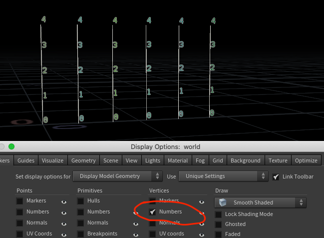
Cool, that's probably exposed as @vtxnum, lets see if its what we want. I'll copy it to @a, and display that alongside the vertex numbers ( @a is in orange, the vertex numbers are in blue, and less points cos its getting a bit crowded):
vex
i@a = @vtxnum;i@a = @vtxnum;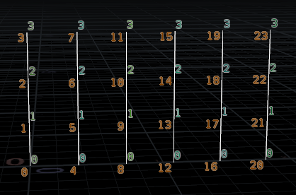
What? Something funny is going on here. It seems like @vtxnum is not the same as display vertex numbers in the viewport.
What we're getting with @vtxnum is the linear vertex number. What's that? Well, if you were to look in the geo spreadsheet and count the number of rows, that corresponds to the amount of points you have. If you jump over to the vertex page of the geo spreadsheet, you could count the number of rows to get the number of verticies you have. If you were to write down those numbers, thats what @vtxnum is, a unique id per vertex.
But but but... that's not what we want! Is there a way to go from that unique id back to the id-within-the-prim?
Of course there is, vertexprimindex! Given a linear vertex it returns the vertex prim number, ie, the index of the vertex within its primitive.
Here I'm visualising the @vtxnum in violet, and vertexprimindex in red. You can see that it matches up with the viewport display of vertex numbers:
vex
i@b = vertexprimindex(0, @vtxnum);i@b = vertexprimindex(0, @vtxnum);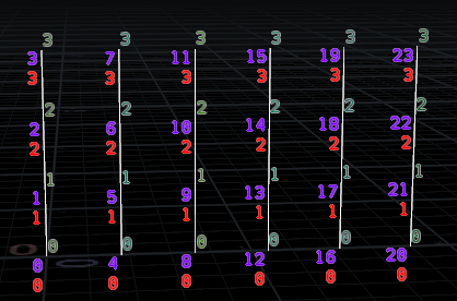
So, to identify the first point per curve, we could now put that into a test and do things, eg:
vex
int vp = vertexprimindex(0, @vtxnum);
if (vp == 0) {
    @group_root = 1;
}
int vp = vertexprimindex(0, @vtxnum);
if (vp == 0) {
@group_root = 1;
}As an aside, you might be wondering why all this complication. The answer is that you have to remember that there's not a 1:1 correspondance between points and verticies. With these simple curves it seems like it is, but think about a polygon sphere, the point at the top and bottom poles will be associated with tens, maybe hundreds of verticies.
What @vtxnum is really doing is giving you the first linear vertex it finds. There are other vex functions to let you find the rest of the verticies associated with a point, if you search the vex functions there's several entries for different ways of moving from points to prims to verts and back again.
If none of that makes sense, you might want to read up on points and verts and prims.
Find the median curve from many curves with vertexindex
Semi-related to the above, say you have many curves with the same number of points, eg curves to represent the arms of an anemone. You want to find the average of all these curves to define a center curve.
Ultimately you want to find the position of the first point of every curve, add and average, set that as the position of your new curve. Then do the same for every matching second point from every curve, then the third, etc.
Layering a bunch of assumptions here, lets say that the curves have no branching, meaning that ptnum will basically be the same as vtxnum for these curve. As such, we split off a single curve, connect it to a wrangle, feed all the curves to the second input, and run this:
vex
int lv, curve, curves;
vector pos;

@P = 0;
curves = nprimitives(1);
for (curve = 0; curve < curves; curve++) {
   lv = vertexindex(1, curve, @ptnum);
   pos = vertex(1, 'P', lv);
   @P += pos;
}
@P /= curves;
int lv, curve, curves;
vector pos;
@P = 0;
curves = nprimitives(1);
for (curve = 0; curve < curves; curve++) {
lv = vertexindex(1, curve, @ptnum);
pos = vertex(1, 'P', lv);
@P += pos;
}
@P /= curves;Reading that through:
- Set @P to 0
- Init some variables
- Get how many primitives are coming from the second input, store as the 'curves'
- loop through from 0 to the total curve count:
- for the current curve in the loop, lookup the vertex number corresponding to our single input curve ptnum
- read that vertex position (lucky for us vex will calculate the current vertex position even though @P doesn't exist for our vertices
- add that to our current point position
- after the loop, divide the position by the number of guides, giving us the average position.
Query image width and height
Download hip: Download file: uv_scale_from_image.hip
vex
string map=chs('image');
float x, y;
teximport(map, 'texture:xres', x);
teximport(map, 'texture:yres', y);
@ratio = x/y;
string map=chs('image');
float x, y;
teximport(map, 'texture:xres', x);
teximport(map, 'texture:yres', y);
@ratio = x/y;The teximport function lets you query a few proprties of an image (full list here: https://www.sidefx.com/docs/houdini/vex/functions/teximport.html ), faster than loading an image into cops and querying that way. This example uses that to scale the uvs of an object, so that the uv's match the ratio of an input image.
Ensure unique names
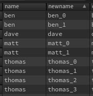
Good question from lovely friend and coworker Ben Skinner. Say we have some primitives with a @name attribute, and several share the same name. How can we make the names unique?
The lazy answer is just append the primnum to the name:
vex
@name += '_' + itoa(@primnum);@name += '_' + itoa(@primnum);Works, but its a bit blunt. What if some of the names have no duplicates, can we leave them unchanged? There's a few vex functions that will identify unique attrib values, here' we'll use findattribvalcount. This snippet will only run the rename if there's more than 1 unique value:
vex
int count = findattribvalcount(0,'prim','name', @name);
if (count>1) {
  @name += '_'+itoa(@primnum);
}
int count = findattribvalcount(0,'prim','name', @name);
if (count>1) {
@name += '_'+itoa(@primnum);
}Also works. But the result is a bit messy, as the primnum suffix will be arbitrary rather than ordered. Ideally if there's 4 prims that share the name 'thomas', they should get the names 'thomas_0, thomas_1, thomas_2, thomas_3'. We can do that with findattribval, which creates an array of the prim numbers. If the length of the array is greater than 1, use find to get the index of that prim within the array, use that as the suffix:
vex
int prims[] = findattribval(0,'prim','name', @name);
if (len(prims)>1){
    int pr = find(prims, @primnum);
    s@name +='_'+itoa(pr);
}
int prims[] = findattribval(0,'prim','name', @name);
if (len(prims)>1){
int pr = find(prims, @primnum);
s@name +='_'+itoa(pr);
}Distort colour with noise and primuv
Download hip: Download file: col_distort.hip
I've tried distorting surface values with noise before but never got it quite right, Jake Rice had the answer (Jake Rice ALWAYS has the answer). Start with curl noise to define the distortion, project back to your surface, lookup colour at that point. Simple, fast, works great.
vex
vector noise = curlnoise(@P*ch('freq')+@Time*0.5);
vector displace = noise - v@N * dot(noise, v@N); //project the noise to the surface
int prim;
vector uv;
xyzdist(0, @P + displace * ch("step_size"), prim, uv);
@Cd = primuv(0, "Cd", prim, uv);
vector noise = curlnoise(@P*ch('freq')+@Time*0.5);
vector displace = noise - v@N * dot(noise, v@N); //project the noise to the surface
int prim;
vector uv;
xyzdist(0, @P + displace * ch("step_size"), prim, uv);
@Cd = primuv(0, "Cd", prim, uv);I tried using another attribute noise sop to get a nice UI for the noise values, but interestingly nothing looked as nice as good ol' curl noise.
itoa and 64 bit precision limits
Someone on discord had an issue that could be summarised as this:
vex
s@test= itoa(2200000000);
// returns -2094967296s@test= itoa(2200000000);
// returns -2094967296This is due to limits of the default 32 bit integer type; values above around 2100000000 will wrap around to negative values.
The fix required 2 things, to swap to 64 bits, which you can do on a wrangle by going to the bindings tab, and changing 'VEX Precision' to 64-bit.
The other is to swap the itoa function for sprintf, like this:
vex
s@test= sprintf('%i',2200000000);
// returns 2200000000s@test= sprintf('%i',2200000000);
// returns 2200000000Random dot patterns
The end goal. So many dots!
The dots vop is nice, but a bit limited, someone asked on a discord how to extend it.
I had a hunch that I could look at some shadertoy code, and port it over to vex. By the time I'd done a super basic setup, Jake Rice had made an all singing all dancing version. Doh.
Still, was nice to pull this back to first principles, thought it'd make a good mini tutorial for here.
Make a grid with say 500x500 points, uvtexture it (with uv's in point mode), append a wrangle.
First, lets visualise those uvs:
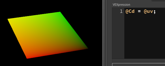
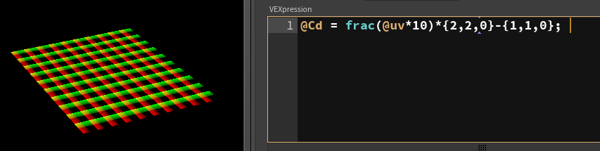
If we want 10x10 dots, lets mult this by 10:
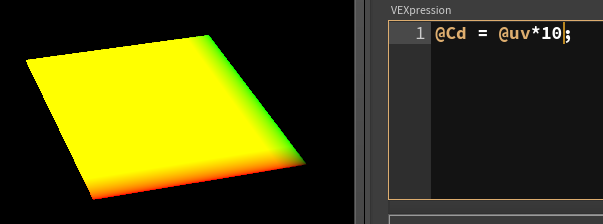
We can use the frac function that strips off anything before the decimal point, so a uv of {8.25,4.12} becomes {0.25, 0.12}. This has the effect of tiling our uv's into mini 10x10 regions:

Each of these mini zones goes from 0 to 1 in uv space. We can measure the length of the uvs, which should give us little circular gradients:
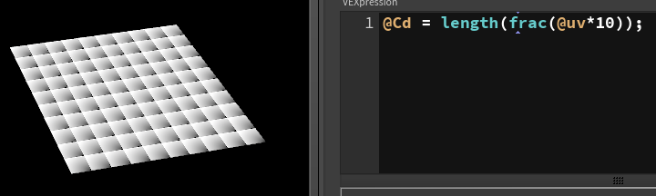
Well, sort of. we're getting a quarter of a gradient, because {0,0} of each tile is in the corner. If we could move it to the center of each tile, we'd get a clean circular gradient.
The center of the tile would be at {0.5,0.5}. To shift these uv's so that the center becomes a value of 0, we multiply by 2, then subtract 1.

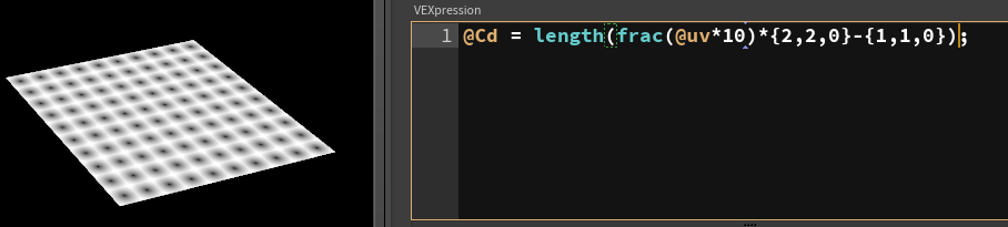
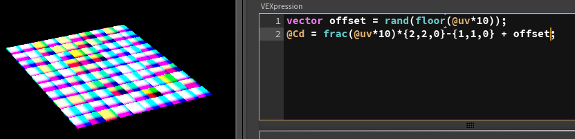
Now if we use this with length(), we should get nice circular gradients:

Huh? It's sort of right, but those values look weird... oh hang on, look whats going on in the geo spreadsheet before calculating length:
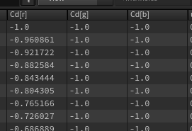
Even though we know uv's are just 2 values, the u and v, houdini always stores it as a 3 value vector, and just leaves the last component as zero. When we copy this to colour and run tha above formula, we're still calculating the blue channel. It has 1 subtracted from it, so blue is -1 for all points. The length of -1 is 1, which is breaking stuff. We have to ensure the blue value is 0 before calculating length. Lots of ways to do this, I chose to be more correct and use vectors for the calculation rather than lazy floats:
Looks the same in the viewport, but the geo spreadsheet now has 0 in the blue column. Calculating the length now looks correct:
Now how to convert this gradient to a dot? We could fit() this, so we say values between 0.5 and 0.6 will become values between 0 and 1, values outside this range will be clamped:
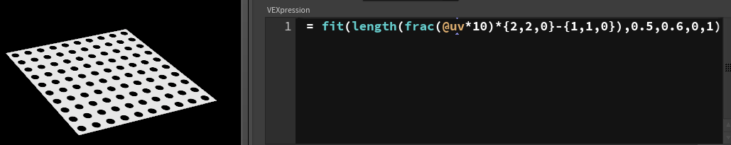
The smooth() function is basically the same, as is fit01(), they just assume the output needs to go to between 0 and 1. Smooth has the extra advantage of a bias function, which you can use to tweak the shape of the gradient edge should you want it. It's very similar to the smoothstep() function in HLSL/GLSL, which can make porting things you see on shadertoy a bit easier. 😃

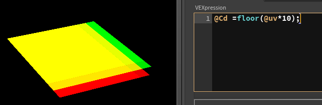
Ok thats regular dots. How can we give them random offsets? Going back to the frac() we did, if frac keeps the value after the decimal point, floor() does the opposite, and keeps the values before the decimal point, eg {7.25, 3.23} becomes {7,3}.
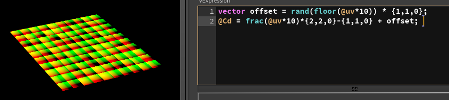
Now that we have a 'flood filled' value per tile, we could feed this to rand(), to get a rand value per tile:

We can treat this as a vector, and add this to the center-offset uv from earlier:
Ahh, bits of blue there, don't fall for that trap again. Make sure to remove any blue:
And now calculate the length and smooth it, how do our dots look?

They're offset, but offset too much and are clipping off the edges of their tiles. The dots are pretty big within their tiles, so we should shrink them to give them more space to be offset. Also the offset values are too extreme, and are positive, so lets zero center them and reduce their range with a fit. As always, gotta make sure the third component is zero'd out, I've used a different tack here and just set it explicitly:
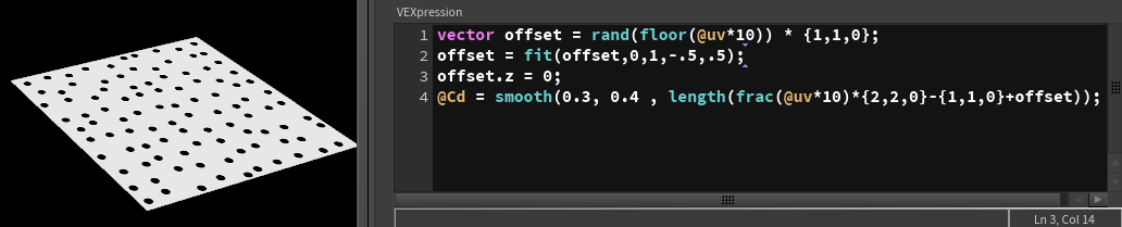
Finally we can swap out the magic numbers for channel sliders, get something nice and interactive:
Here's the full code:
vex
int tiles = chi('tiles');
float rand = ch('rand');
float start = ch('dotradius_start');
float end = ch('dotradius_end');
vector offset = rand(floor(@uv*tiles)) * {1,1,0};
offset = fit(offset,0,1,-rand,rand);
offset.z = 0;
@Cd = smooth(start, end , length(frac(@uv*tiles)*{2,2,0}-{1,1,0}+offset));
int tiles = chi('tiles');
float rand = ch('rand');
float start = ch('dotradius_start');
float end = ch('dotradius_end');
vector offset = rand(floor(@uv*tiles)) * {1,1,0};
offset = fit(offset,0,1,-rand,rand);
offset.z = 0;
@Cd = smooth(start, end , length(frac(@uv*tiles)*{2,2,0}-{1,1,0}+offset));If you wanna take this further, here's some exercises to try:
- Can you do random sized dots?
- Can you give them random colours?
- Can you use a for loop to get layers of dots that overlap?
Random dots with overlaps on youtube
As an experiment I recorded a video tutorial to take this to the next level, answering some of the questions I posed above. You can find it here:
https://www.youtube.com/watch?v=XZTFBRj--CY
Further learning
JoyOfVex if you haven't done that already.
Juraj Tomori has written an amazing guide go read it right now: https://github.com/jtomori/vex_tutorial
Sidefx have a cheat sheet similar to this one, but it assumes a lot of prior knowledge. If you've made it this far down the page you're probably ready for it, and it points out a lot of edge cases that I've glossed over:
https://www.sidefx.com/docs/houdini/vex/snippets.html
The 'bees and bombs' thread on odforce is a bunch of practical(ish) visual examples; lots of self contained looping animations created (mostly) in vex. Be sure to check out the threads at the end, Robert Hodgin has cleaned up most of my earlier setups in that thread so that they work properly in H16:
http://forums.odforce.net/topic/24056-learning-vex-via-animated-gifs-bees-bombs/
Ryoji CG has a handy collection of wrangle snippets:
https://sites.google.com/site/fujitarium/Houdini/sop/wrangle
The wrangle workshop isn't bad, but if I'm gonna critique moves a little slow (I'm also super impatient and prefer text to video, but thats me...)
Shadertoy is a great place for inspiration. The code isn't vex, and a lot of the files use techniques that don't directly map onto Houdini, but even then its handy to see a visual example of a technique you might want to implement, and the core algorithm can often be remapped to vex easily enough:
Processing, various javascript graphics libraries, older actionscript, all great to steal ideas from.