Blender Geometry Nodes ​

The first Cgwiki Cinematic Universe in 2002 or so was like Marvel pre Iron Man, no-one cares.

The second CCU started in 2014 when I made a bunch of examples for the Maya SOuP plugin.

The third CCU started in 2015 when I ported those examples to Houdini, kicking off big interest in this site, lots of notes, what most people think of as 'cgwiki'.

Well its 2025, the forth CCU is here: porting the SOuP notes to Blender geometry nodes.

Brace.

Basics ​

This'll start more verbose as I try to explain the similarities/differences to Houdini, and get less verbose the deeper we go.

Shortcuts and assumed knowledge ​

• shift-a - like tab in houdini, will bring up a menu to add things.
• g - grab, same as translate. when active, x, y, z will constrain in that axis, and shift-x, shift-y, shift-z will constrain on that plane.
• k - set keyframe, will bring up a menu of options, subsequent pressings of k will be focused on the last keyframe option you chose
• spacebar - toggle playback
• shift - left arrow - jump to first frame
• n - toggle the panel on the right. Basically an extra panel of properties that overlays in the current editor.
• t - toggle the toolbar for the current editor on the left.
• a - select all
• h - hide, or toggle collapsed mode in the node editor
• opt-h - unhide
• m - toggle a node's mute state, like b to bypass in houdini.

Attribute transfer and position ​

Download blend: gn_transfer_position.blend

Transfer the position of locator (empty) to the points of a grid, with a smooth falloff.

Setup ​

1. Create grid a grid, use the dialog in the lower left of the viewport to set divisions
2. Create empty, which is the same as null or locator in maya/houdini
3. Grab the empty and move on the ground plane (g, shift-z), move to one side of the grid
4. k to keyframe, set 'location'
5. Move to frame 50
6. Move the locator to the other side of the grid, keyframe
7. Playback the motion to ensure it feels appropriate, drag keyframes in the dopesheet to adjust timing.

Get into geo nodes ​

1. Select the grid, click Geometry nodes in the top toolbar to get into the geo node layout
2. In the network editor, click New at the top to start a new geonode network

Here you should see 2 nodes connected with a green line. This is the flow of data like in sops, but left to right. Lets setup the transfer, and pull in the locator to the graph so we can query its information.

Geo node setup ​

1. Drag the empty from the outliner into the geo node network. This will create an Object Info node we can use to query its translation data.
2. shift-a in the network view, start typing 'position', when its found, hit enter, then l.click to drop it into the network.
3. shift-a, create a distance node
4. Drag from 'location' on the Object Info node, to the first vector input of the distance node.
5. Connect Position.Position to the second vector input. The output of this will be the distance of each point on the grid to the empty.
6. shift-a, create a map range node
7. Set 'from max' to 0.6
8. Create a float curve node
9. Connect Map Range Result to Float Curve Value
10. Add 2 points to the curve to give it a S-curve
11. Create a mix node
12. Change its mode from 'Float' to 'Vector'
13. Connect ObjectInfo.Location to A
14. Connect Position.Position to B
15. Create a Set Position node
16. Connect GroupInput.Geometry to SetPosition.Geometry
17. Connect Mix.Result to SetPosition.Position
18. Connect SetPosition.Output to GroupOutput.Geometry

Notes ​

Geometry nodes (shortened to geonodes or GN from now on) can be vops style or sops style within the one network. Generally when results have to be pushed back onto geometry, those nodes require a geometry input and output, represented by a green wire. Other nodes that are more atomic (vector add, read attributes etc) won't require the green wire.

Position is the same as @P, obviously. Object Info is similar to an OpInput call. Set Position in this case is closest to a Bind Attribute.

You might notice the end result looks messy with all those parameters on the nodes, its cluttered if you're used to minimal Houdini sops nodes:

You get used to it, but there are other ways to tidy this up, as shown in the video loop at the start of this post. All the nodes have a expand/collapse button in their upper left corner, you can also marquee select all the nodes (or just tap a to select all), then tap h to toggle the expanded/collapsed state. Tap n to bring up the network panel (like hitting P in Houdini), and choose the 'Node' tab. Now you have something much closer to Houdini, select a node, its parameters appear in the side panel.

Much tidier!

The float curve node acts like its in 'cook on mouse up' mode, other nodes with float parameters update immediately. I discovered this while dragging curve editor dots around and wondering why the geometry wasn't updating... I just discovered that if you drag the X and Y sliders at the bottom of the graph for the selected dot, that DOES update in realtime.

m will toggle a node mute, like hitting b to bypass in Houdini.

shift-rmb-drag over a wire will insert a dot.

ctrl-x/cmd-x on a node will delete it, and try to cleanly update the wires so the network is still connected. This also works for deleting dots.

Node colours broadly correspond to functionality.

• Red: An input, eg a geometry attribute, scene time, uv's.
• Blue: A 'doing node', eg maths nodes, comparisons
• Green: Modifying geometry, eg setting attributes, changing subdivisions, applying materials.

Attribute transfer and Color ​

Download blend: gn_transfer_colour.blend

Transfer colour of an empty to the points of a grid, with a smooth falloff.

The network change is relatively small, but getting the colour attributes setup and visible in the viewport takes a bit of work.

Setup ​

1. Select the grid, in the main Properties panel (right side of the UI), open the Data tab (upside down green triangle)
2. Expand 'Color Attributes', click the + button to add a new attribute
3. In the dialog leave its name as 'Color', and set the colour to red.
4. In the viewport, ensure you're in solid mode (upper right of the viewport, the solid circle)
5. Click the dropdown on the right of the shading modes
6. Set object colour to 'Attribute', the grid should now be red.

Now back to geonodes...

Swap position for color ​

1. Ensure you're starting with the previous setup
2. Select the Set Position node, ctrl-x/cmd-x to delete it but keep the wires connected
3. shift-a, 'store named attribute', drop it onto the green wire, set its mode to 'Color', attribute name to Color (it's the blank parameter, and it will bring up a list of available attributes when clicked). The grid will go white, as thats the default value on this node.
4. Disconnect the two purple inputs on the mix node, we'll use it to mix colour instead.
5. shift-a, color, that will create a color constant node. make it green.
6. connect it to the first purple input of the mix node, and then the mix output to the value input of the store named attribute. If you scrub the timeline, the grid will be green where the empty is, but black elsewhere. Lets connect the red Color attribute that's on the grid.
7. shift-a, 'named attribute' node. change its mode to 'Color', and then name to 'Color'
8. Connect the named attribute yellow output to the second mix input.
9. Scrub the timeline, see that its now mixing the red of the grid with green where the empty is.

Notes ​

Houdini uses @Cd, Blender uses 'Color'. It's not visible by default in the regular viewport, so you have to tell it to load it.

The network simply reads @Color with the named attribute, and writes it back to the geometry via the Store Named Attribute. We'd already done the work of the mix logic, may as well reuse it!

Waves ​

Download blend: gn_waves.blend

This is straight up vops really, no surprises:

1. Add a grid, fresh geometry node network.
2. Add a Set Position, insert it into the green geometry wire stream
3. Add a Position node and a Scene Time node
4. Add a Separate XYZ and a Combine XYZ
5. Connect X -> X, Y -> Y. Z we'll modify to make waves.
6. Add a Sine node, connect SeparateXYZ.Y to its input, and its output to CombineXYZ.Z
7. Connect CombineXYZ.Vector to SetPosition.Position.
8. That's a giant wave. Add a Multiply node, insert it before the Sine. Add another Multiply node, insert it after the Sine
9. The first multiply controls frequency, the second controls amplitude.
10. To make it animate, add an Add node, insert it before the first multiply, and add SceneTime.seconds to Y. If you play the time line (spacebar), the waves will animate.

Notes ​

You get used to Z up, stop whining.

I labelled the nodes, hit n to bring up the node panel if its not visible already, select a node, change its label parameter.

Vex and wrangles don't exist ​

They don't exist in geo nodes, it's the thing I miss the most from Houdini. As a consequence geonodes can feel a bit Unreal blueprinty at times, you're putting down 8 nodes when you know it should be a 2 line vex script, but watchagonnado?

There's been a few attempts at a basic expression system (think like the Nuke expression node), and I'm aware of one python module to let you write 'in code' and it generates nodes for you. But really, neither are quite like Vex.

It's interesting in that Sidefx themselves are kind of sidestepping Vex of late and pushing OpenCL, and Apexscript. I understand making Yet Another Language is a big ask, but man... I'd love a wrangle...

If statements ​

Download blend: gn_if.blend

More contrived examples, mainly to show different ways of managing control flow in SOuP/Houdini/Geonodes.

Many nodes have a Selection input, the pink colour tells you its a Boolean. This is analogous to the group parameter in Sops, if its true for the given point/edge/face, that element is modified by the node.

Here I have an Index and a Scene Time node. They're modulo'd, then that result is compared to 0. If it's true, then that's passed as a selection to the Set Position node to move it up on Z.

Rays ​

Download blend: gn_rays.blend

Use an Arctan2 node connected to a Sine node to generate radial rays, with extra nodes to control animation, frequency, amplitude.

Main thing to notice here is a wiring style I've seen a few times; stacking nodes. To save horizontal space, it's common to collapse nodes that belong together, and stack them vertically, with the wires zig-zagging behind them. You can subnet/group nodes, but this style is useful when you just want to save a bit of scrolling.

Group inputs (promote parameters) ​

Download blend: gn_group_input.blend

So far I haven't feel the need to wrap up my UI's in the way I do with vops, but the functionality is there. Simply drag anything you want to promote to an empty slot on the Group Input node (equivalent to the global inputs in vops), and it becomes available to edit from the modifier panel.

To give it a nice name, hit n to display the node panel if its not there already, jump to the Group tab, and the inputs are listed in the Group Sockets section. Double click an input to rename.

If you've looked at the rest of this site you know I like to keep my node layouts clean; having everything wired to the one group input can get a little tangly, here's my attempt to keep this clean. You can reorder the group inputs by dragging and dropping in the group sockets list, which I've used here to make the wiring as tangle-free as possible.

Another way is to simply have multiple group input nodes; all sockets appear on all group inputs, so you can keep things localised, less long wires:

Move Edges ​

Download blend: gn_move_edges.blend

Geonodes is the same as Houdini and SOuP in that it can't directly move edges. There are some nodes that can read attributes, do certain manipulations that Houdini can't, but moving edges requires the same tricks.

This example has a couple of interesting things. There's more green nodes, which broadly correspond to sops style operations; creating, modifying, deleting geometry. Rather than use the group input geometry, this uses a grid node to create it parametrically.

This is another common design pattern I've seen with geonodes, start with any dummy mesh, then skip the group input so it's never seen or used. This can sometimes be confusing, as some parts of Blender will still refer to the original mesh instead of the geonodes output. If you disable the geonodes modifier in the modifier list, the original geo will return. Similarly if you go into edit mode, you'll see the original geo, some python calls to query the mesh will see the original geo etc.

If this happens, you might have to bake the geonodes modifier by using the Apply option in the modifier dropdown.

The logic to create the strips uses the same trick as in SOuP and Houdini; it uses modulo based on the amount of grid divisions to tag every other row and delete it. By promoting the grid x divisions to a group input, it can then drive the modulo divisor, and the y divisions, so its all parametric and cool.

To fake moving the edges, this setup uses sine waves based on the point index. If a point's index isn't even, it subtracts 1 from its index, so it basically moves the same as its neighbor, giving the illusion that edges are moving.

To make the weave pattern, there's more green sop style nodes, a transform to rotate the strips 90 degrees, a join to merge with the original orientation, and a shade smooth to fix the faceted normals.

Attribute transfer from shape ​

Download blend: gn_transfer_shape.blend

Can't help thinking there's a better way to do this. If you know a way, get in touch!

Background context ​

I had to go back to the first SOuP example to remember what this was meant to demonstrate, then why the Houdini one veered away, and then if there was anything useful to show here; I think there is.

SOuP made heavy use of gizmos to drive setups, so you'd get sphere gizmos, capsule handles, box handles etc. They'd all have an SDF style weight associated with them, which could then drive colour blends, attribute blends, whatever else you need.

As such, the base of this SOuP example was using a capsule gizmo to transfer its weight into a grid, and then do something with that weight, which was generate waves that followed the shape of the capsule.

Houdini doesn't have capsule gizmos as far as I know. In an attempt to keep it simple I used an attribute transfer sop and a line with many points to represent the capsule. By setting appropriate blend and distance values, the transferred weight looked enough like a capsule SDF to work, make waves, done.

Elsewhere on this site I tried to recreate an attribute transfer in raw vex/vops, and its harder than I expected. Recreating the blend/blur slider of the attribute transfer sop requires for loops or point cloud fiddle stuff.

This implementation ​

So now the geonodes version. Early builds of geonodes had an attribute transfer node, but as Gemini informs me, "Transfer Attribute node was removed in Blender 3.4 and replaced with a set of ... different nodes based on the sampling method (index, nearest, or nearest surface)."

Ok sure, but its suggestions of how to get the same effect weren't great. In the end it was easier than I thought, and plays to the strengths of how geonodes is a hybrid of sops and vops.

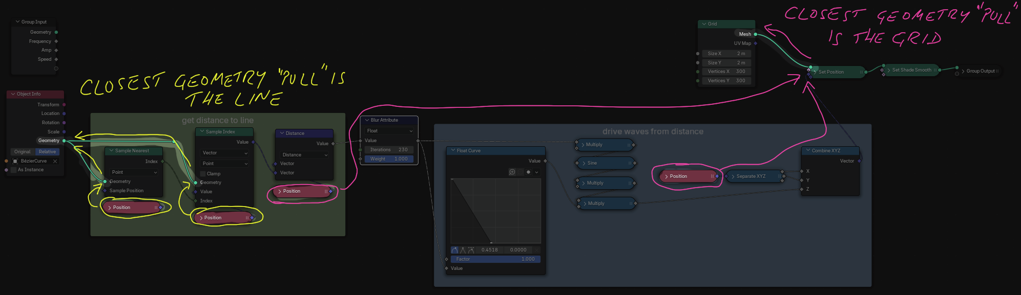
For each point on the grid, get the index of the nearest point on the target line. Get the position of that index, then measure the distance from grid point to that point. That's our capsule falloff.

The rest is straightforward, sine from that distance, use it as the height, set the freq and amp to taste.

This works, but if you only have a few points on the line, you'll notice steppy artifacts:

Luckily you can just throw in a Blur Attribute node after the distance calculation, and crank it until it looks smooth again.

Position vs position vs position ​

If you look at the setup you can see I have several position nodes. The first two refer to positions of the line points, while the second two refer to positions of the grid points. But look closer; if this were Houdini, you'd explicitly say 'refer to geo input 0' or 'refer to geo input 1', but here I don't.

This took a little getting used to, but geonodes 'pull' their context from the nearest downstream node that has a geometry input. What does that mean?

The first two position nodes are connected to the sample nearest and sample index nodes, they both have their geometry input from the line. Therefore, those position inputs refer to the line.

The closest downstream geometry input after the 3rd and 4th position nodes is right at the end of the flow, from the 'Set Position' node. Because the Set Position has its geometry input from the grid, these position attributes refer to the grid.

As I keep saying, doesn't take long to get used to this. 😃

Simulation zone ​

Download blend: gn_transfer_position_simulation_zone.blend

Basically the same as a solver sop, with less of the annoying context diving and viewport pinning.

The core setup is adapted from the first example on this page, the keyframes on the empty are removed, its parented under another, and its rotateZ has the expression #frame*0.1, so it spins in a circle.

The geonode network gets the distance from each grid point to the empty, and uses a Float Curve (a chramp for you Houdini folk) to reverse it, and give it a soft falloff from 0.2 at its center to 0 a short distance away.

The new concept here is the Simulation Zone.

shift-a and look for Simulation, it creates a 2 node region similar to a for loop in vops. The idea is identical to a solver sop; it reads its inputs on frame 1, for other frames it reads from the last simulation node as a feedback loop.

To get this fade effect requires adding the falloff to the previous frame (the first add node), clamping the result to stop it running away (the clamp node), then reducing the total falloff by a fixed amount on every frame to do the fade (the multiply node). Playing with the various values will affect the height, shape, speed of the fade.

Attribute transfer from fancy shape ​

Download blend: gn_transfer_shape2.blend

The original intent here was to show how to move from using SOuP's gizmos to using meshes. Porting the examples to Houdini (and now to geonodes) where everything is meshes and points means the attribute transfer method is unchanged from the earlier example.

What was more interesting here was replicating the animated cylinder motion. I think for the houdini version it uses a tube (ie cylinder primitive), that gives you separate radius controls for the top and bottom.

The cylinder primitive in geonodes doesn't give you this, so I thought I'd use a line, give the points an animated pscale (or whatever the geonode pscale equivalent is), then sweep it into a tube.

This was the first time in a while where geonodes wrong footed me. I've been using hair curves a lot lately, they use 'radius', so I thought I could just go curve -> set radius -> Curve to Mesh (which takes a profile curve as another input, so here its using a circle).

It didn't work. Did some digging, seems it used to be this way, but was changed. The Curve to Mesh node has a Scale input, it's diamond input shape implies it can understand a per-point input. The position node for example, it has a diamond output, the Separate XYZ node has a diamond input, so both understand that whatever operation they do, it operates per point. I guess the analogy here is Hoduini's polyextrude node and its zscale input, it understands that it's read per point.

Anyway, to generate this per-point scale I use a Spline Parameter node, that gives you access to the 0-1 factor of each point along the curve. This is animated with Sine and Multiply nodes in the usual way, then passed to a map range to remap it from (-1,1) to (0.2, 0.5), and that is connected to the Scale input.

Selections ​

Download blend: gn_selections.blend

Sops in Houdini often use groups to define what should be modified. Selections in geonodes are basically the same thing. A lot of nodes will take a Boolean pink selection input, only elements that have this value as true will be modified.

Unlike Houdini, it's not hardcoded to @group; its whatever attribute you choose to connect.

There's no selection node in geonodes, meaning there's no easy way to define a selection by a bounding input that I can see. Instead here I use 2 raycast nodes, and use the 'Is hit' boolean output, when raycasting from the grid to the animated monkey. One node raycasts up, the other down, then I use a boolean 'AND' node to reduce to only points where both up and down raycasts are true.

This boolean is sent directly to the selection input of a Delete Geometry node, job done.

Or is it?

The monkey-hole left behind is quite jagged, I figured this would be a good use case for another selection.

The same AND result is used to drive a switch, that outputs a float value of 0 if false, and 5 if true. This is then blurred, and run to a float comparison. This has the effect of expanding the monkey intersect zone, which is stored as @smoothme, and because of the when the geometry wire is used, is stored before the delete operation.

After the delete, the @smoothme attribute is read, and that itself is used as a selection on a Set Position node, which sets a blurred position. This has the effect of smoothing the monkey hole.

This is convoluted of course; there's boolean geonodes, and probably tidier ways to achieve this effect, but I hope its a good way to explain some selection tricks.

Selections persistent via simulation zone ​

Download blend: gn_selections_persistent.blend

Relatively minor tweak to the previous example gives persistent selections.

Both boolean values we're interested in (the raw raycast result and the blurred/expanded one) are run to a simulation zone. On each frame the current result is compared to the previous frame with a boolean OR. It basically means once a point has its boolean value set to True, it stays True for the rest of the frame range.

Delete with slider ​

Download blend: gn_delete_with_slider.blend

Mildly interesting example of doing a comparison on index, and feeding that selection directly to a Delete Geometry node. What's more interesting is...

Visualise point numbers ​

It took me a while to work out how to enable point numbers, writing it down (and put it in the video) so others can find it more quickly than I did.

It's not a simple button on the side of the view, it's more like the viewer node in Nuke, or the 'x' to preview nodes in the Houdini material editor. It requires you to connect both geometry and an attribute to view, and twiddling the overlays.

1. Create a Viewer node
2. Connect the index node to the value input of the viewer
3. Connect a geometry output of the Delete Geometry node to the geometry input of the viewer.
4. Enable the viewer if its not active by tapping the little monitor icon in the top left
5. This will show the connected value as a colour, but we want to see the actual text value.
6. Go to the overlays menu of the viewport (top-right, two overlapping circles).
7. In the viewer mode options 2/3 the way down, turn off Color Opacity, turn on Attribute Text.

Tada! Point numbers!

Instance with effector ​

Download blend: gn_instance_effector.blend

Instance on Points is the geonodes version of copytopoints. Now that I'm aware of the pscale, zscale, polyextrude sop style behavior, this had less surprises for me.

Should in turn have no surprises for you, it was just a nice exercise to try and recreate the look of the Houdini example. A spherical Empty is used to drive the setup, relatively straightforward things in here to set the falloff shape, scale the cubes, preview colours with a Viewer.

Instances on animated geo ​

Download blend: gn_instances_on_animated_geo_stable.blend

The more common workflow for copy to points, ie scatter some points, then copy geo.

In geonodes scatter is Distribute Points on Faces, and has the same issue that scatter in Houdini does; if the input geo is animated, the points will also animate and jump around.

The fix is also similar to Houdini; generate the points on a static mesh, then interpolate attributes from an animated state of the mesh using a UV lookup. A few things to be aware of:

• There's no intrinsic UVs
• There's no attribute interpolate node
• When setting up the interpolation yourself, its one attribute at a time, no wildcards.

In place of intrinsic UVs, most similar workflows in geonodes assume you have some regular UVs setup on your mesh. Because the input here is a procedural grid we have no UVs, but the UV unwrap node seems to work fine. Interestingly you treat it like reading position or index or normal; its a node with a simple vector output, which you have to explicitly write into your geometry with a Store Named Attribute.

Instead of attribute interpolate, you do it like you'd do in vex, with a uv lookup. The node is Sample UV Surface, it takes the mesh to sample as input, the attribute you want to lookup, and the UV attribute.

Note the slightly confusing flow of data, it has a single geometry input, the geometry to sample from. Like earlier, the geo the data is pushed to is the closest downstream node that has a geometry wire. In this case for sampling position, it comes from the downstream Set Position node, which is the scattered points. Similar for the normals, its closest downstream node with a geometry input is the Instance on Points node, which also has the scattered points as its input.

The attribute interpolate node in Houdini helpfully defaults to a wildcard * for all attributes, so the scattered points inherit all attributes from the grid. Sample UV Surface can only do a single attribute at a time.

Minor final note; if the grid divisions are too low, you'll still see popping. I suspect this is due to triangulation; the animated noise is distorting the quads enough that the quad triangulation flips. In practice you'd probably never use a grid layout this low res.

Btw, if the lack of implicit/parametric UVs bothers you like it bothers me, upvote this please. 😃

https://blender.community/c/rightclickselect/7WP1/

Attribute from Texture ​

Download blend: gn_attribute_from_texture.blend

The idea is simple, the handful of techniques in here is interesting.

Relative bounding box ​

A favourite Houdini trick of mine is to modify points based on their position relative to the mesh bounding box. There's a vex call to do this, in geometry nodes I can use the Bounding Box node, and connect its min and max output to the From Min and From Max of a Map Range node. This is stored as @bbox.

I then read this directly into the next stage, and use it as fakey UV's on an image texture. That value is stored as @Color.

Group ​

To do the wave animation, I did the same input -> mult -> sine -> mult -> position thing as in a few prior examples but got tired of the messy stacked nodes, so introduced a new concept here, Group.

You can select a bunch of nodes, and from the menu in the geonode network editor choose Node -> Make group (or press ctrl/cmd-g).

You'll immediately be thrown into a new context with group input and group output nodes, and the nodes you selected in the middle. This is very similar to a subnet in Houdini. The tab key will toggle you in and out of the group.

You can promote parameters here the same as promoting parameters to the modifier stack. Connect wires to the group input node, and rename them from the n key menu -> 'Group' tab (while inside the group). When you jump out, those parameters will be available on the top of the group.

When outside of the group, select it and give it name from the n menu, Node tab. This group is now a reusable asset; you can hit shift-a, search for that name ('Animated Sine' in my case), and its available to be reused. Handy!

Colour ​

Finally here I had to work out how to actually display the colors. I instance circles onto the points of the grid, but they won't inherit colour by default. Instances act as instances, and will implicitly all share the same colour attribute. Appending a Realize Instances node is essentially the same as unpacking, and their colour becomes available.

Except that you still can't see it. 😃

To see it in the viewport you either need to connect to a Viewer. To render it in Eevee or Cycles requires creating a material that reads the Color attribute, and then use a Set Material node in geonodes to assign it.

Eyeballs ​

Download blend: gn_eyeballs.blend

I remember feeling very smug when I worked this out in Houdini and thinking 'Aha, I think I get this'. Nice to get that same feeling with geonodes.

The eye dart animation comes from a noise texture, the animation transition comes from a sine wave clipped and retimed with a float curve.

Walkers ​

Download blend: gn_walkers.blend

Same idea as the Houdini example on making lines procedurally.

• scatter points on the ground
• scatter less points at head height and wiggle them
• draw lines from the closets ground points to the head points
• wiggle the lines a bit, attach a sphere for a body.

This is where the lack of coding becomes a bit of a bore; if I were to do this in Houdini today I'd probably do a nested vex/pseudocode loop like

for headpt in headpoints:
    groundpoints = 8 closest groundpoints:
    for groundpt in groundpoints:
        addline(headpt, groundpt)

for headpt in headpoints:
    groundpoints = 8 closest groundpoints:
    for groundpt in groundpoints:
        addline(headpt, groundpt)

Funny that I didn't read the original houdini entry until doing this little write up, and i complained back then in exactly the same way, 'code is easier for ths kind of thing'. 😃

Fully exposed loops with nodes get messy and hard to follow, so here I've used nested groups to keep it manageable. The topmost loop iterates through each head point, and calls a 'Make Legs' group. If you tab into that group, it finds ground points that are less that 1.9 units away, and calls another group, 'Connect Points'.

Connect points is a repeat zone (a for loop), that takes a start and end position, and creates 4 interpolated points between those positions, as well as a final point for the end position, and the uses the handy function Points to Curves to connect those points into a curve. I'd been looking for an equivalent of the add sop from houdini to convert points to lines, this is the one.

Like doing for loops and iterations in sops and vops, the exact wiring and layout of these loops can be a bit confusing at first, but makes sense in the end. Also tabbing out of nested groups is a mild pain, I've worked out its best to set focus on the group input node first, then tab should take you up and out.