Appearance
Joy of Vex Day 7
Using the other inputs on wrangles, do things to geometry based on other geometry
Minpos
You might have used the ray sop before, minpos is the vex equivalent of that; give it a position, and some geometry, it will return the closest position on the surface of that geometry. To do that will involve a few new concepts:
Keep the grid on the first input, connect pig to the second input of the wrangle, try this:
vex
 vector pos = minpos(1,@P);
 float d = distance(@P, pos);
 d *= ch('scale');
 @Cd = 0;
 @Cd.r = sin(d);
vector pos = minpos(1,@P);
float d = distance(@P, pos);
d *= ch('scale');
@Cd = 0;
@Cd.r = sin(d);Set the scale slider greater than 1, you should get pig shaped waves! Whats going on here?
A lot of vex functions take a number or string as the first input. minpos is one of these, you give it a position, it returns the closest position on the surface of some geometry.
But what geometry? Thats what the number is for. The inputs on a wrangle are numbered 0 1 2 3. The first input (0) is the one that vex will process by default, as we've done in all the examples so far. So minpos(0,@P) would look at the geometry on the first input (ie our grid), but here we're using minpos(1,@P).
To write out whats going on here in long form,
vex
vector pos = minpos(1,@P); vector pos = minpos(1,@P);means
for each point on the grid, find the closest position on the pig, and store that in variable 'pos'.
Why do I keep writing position in italics? Because I want to make clear that its functioning like a ray sop snap to the pig, its NOT the @P of the closest point on the pig. Eg, if were to find the closest position on a 4 sided poly that intersects the grid, vs the closest point position on that poly, they're two different things:
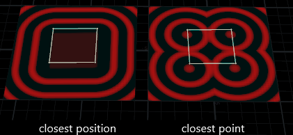
See how by finding the distance to the closest position on the poly, we get an outline representation, like an SDF if you've dabbled in volumes, while finding the distance to the closest point gets what we've had before, a radial distance directly to a point.
The rest is as we know it, a sin wave driven by this distance will make pig waves.
Or give it a box, box waves. Or squab waves etc.
Nearpoint and point
That gif of course leads to the question... what if we want that? Or another thing that happens a lot is that you need to read an attribute from a point in some other geometry.
The non-vex way would be with an attrib transfer sop, so you'd have 2 pieces of geo, and you tell it what attributes you want transferred based on a distance and blend threshold from one to the other. Lets do the vex version.
So as a preamble, think about what we need.
- We'd need to find the id of the closest point in that other geometry from our current @P, then
- We'd need to query that point for the attribute we want.
Item 1 is handled by nearpoint. Item 2 is handled by the point function. Time to test this.
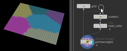
Create a scatter sop after the switch, set it to 6 points, append a colour sop in random colour on points, and connect it to input 1.
vex
 int pt = nearpoint(1,@P);
 @Cd = point(1,'Cd',pt);
int pt = nearpoint(1,@P);
@Cd = point(1,'Cd',pt);So as we've described, nearpoint here takes our current grid @P, and looks at the geo from input 1 to find the closest point, and returns its @ptnum, which we store as pt.
Then, we again query input1 using the point function, asking it what is the colour of the the point that has a @ptnum of 'pt', and we set our current grid point to that colour.
You'll get a pattern that looks like voronoi fracture, because that's exactly what you've made; voronoi cells are a map of the what the closest point is from a sparse number of points (the scatter) to our geo (the grid). The cell lines are where the distance to the distance to the 2 nearest scatter points are the same.
An aside on the point function
You might be wondering why the point function is formatted as
vex
point(1, 'Cd', pt); point(1, 'Cd', pt);rather than
vex
point(1, '@Cd', pt); point(1, '@Cd', pt);or even
vex
point(1, @Cd, pt); point(1, @Cd, pt);The last can be explained easily, @Cd without quotes would be expanded to our current point's colour. Because we have no colour (or even if we did), it would become
vex
point(1, {0,0,0}, pt); point(1, {0,0,0}, pt);So that's not asking for the other point's color, its just stuffing a vector into a function for no reason, its nonsensical. So we have to somehow protect the attribute name we're interested in from being swapped for a value, hence its wrapped in quotes to keep it safe.
Why its 'Cd' and not '@Cd' is less easy to explain. The @ syntax is specific to wrangles, if you look in vops you see they don't use that prefix. Internally attributes are just plain names, the @ is a shorthand so wrangles know when you're referring to attributes vs referring to local variables. As such, the point() function, which is much older than wrangles are, doesn't use @'s.
That said, it feels like it should be a relatively simple thing for the function to read '@Cd', quickly strip the @, and carry on. Lobby sidefx if this interests you. 😃
Visualise the voronoi cell distances
Back to coding!
Regarding how the voronoi cells work, we can visualise the distance to the nearest scatter point by putting it into @P.y; the cell edges should end up being the same height:
vex
 int pt = nearpoint(1,@P);
 @Cd = point(1,'Cd',pt);
vector pos = point(1,'P',pt);
float d = distance(@P, pos);
@P.y = -d; int pt = nearpoint(1,@P);
@Cd = point(1,'Cd',pt);
vector pos = point(1,'P',pt);
float d = distance(@P, pos);
@P.y = -d;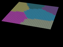
opinput
Say you had 2 identical grids, and one has been deformed by a mountain sop. If the flat grid is fed to input0 of a wrangle, and the mountain'd grid is fed to input1, you can copy the positions of the deformed to the flat with this bit of code:
vex
@P = point(1, 'P', @ptnum); @P = point(1, 'P', @ptnum);So that looks up point in input1 that matches the current point id, gets its position, and assigns it to @P.
In this situation, where you're looking up attributes between two pieces of geo that have matching point counts and layout, there's a shorter method:
vex
@P = @opinput1_P; @P = @opinput1_P;Well, sort of shorter. So you replace...
vex
@ @with...
vex
@opinput1_ @opinput1_...and it will lookup the attribute you specify from that input. It's fine to use either method, in these tutorials you'll find I'll use them interchangeably. To my eye the opinput format is a clear indicator when I come back to the code later that says 'ah, I'm doing matching between geo', whereas point() can refer to any other point, so I'll usually reserve it for that use case.
Also there's meant to be a performance boost for using opinput because its a direct lookup, while with point you're incurring the cost of calling a function. In practice I've never seen much of a difference, in fact some folk have run tests and found point() to be faster. Style wise the @opinput_ thing can look a little messy, especially when embedded into longer functions, if I'm trying to make things look readable I'll assign things to variables first, keep it tidy:
vex
 vector p1 = @opinput1_P;
 vector cd1 = @opinput1_Cd;

 @P = p1;
 @Cd = cd1;
vector p1 = @opinput1_P;
vector cd1 = @opinput1_Cd;
@P = p1;
@Cd = cd1;Exercises
- Pull the following wrangle apart, set the chramp to mostly flat, with a thin triangle in the middle, lots of divisions on the grid, and feed around 8 scattered points to the second input of the wrangle:
vex
 int pt = nearpoint(1,@P);
 vector pos = point(1,'P',pt);
 float d = distance(@P, pos);
 d *= ch('scale');
 d += rand(pt);
 d -= @Time;
 d %= 1;
 @P.y = chramp('pulse',d)*ch('amp');
int pt = nearpoint(1,@P);
vector pos = point(1,'P',pt);
float d = distance(@P, pos);
d *= ch('scale');
d += rand(pt);
d -= @Time;
d %= 1;
@P.y = chramp('pulse',d)*ch('amp');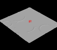
prev: JoyOfVex06 this: JoyOfVex07 next: JoyOfVex08
main menu: JoyOfVex