Appearance
Joy of Vex Day 12
arrays, nearpoints
Arrays
Arrays are lists of values. A vector is a specialised kind of array, helps to do a quick preamble on manipulating vectors before jumping to arrays.
To define a vector you usually use curly brackets:
vex
vector myvector = {1,2,3}; vector myvector = {1,2,3};And to assign it to an attribute, you prefix v before the @:
vex
v@a = {10,12,100}; v@a = {10,12,100};To read values of an array you can use the dot notation, using xyz or rgb:
vex
float foo = @a.x; // will return 10 float foo = @a.x; // will return 10Or another way is to use index notation. The vector elements start at 0, and you use variable[index]:
vex
float foo = @a[2]; // that's asking for index 2, which will return 100 float foo = @a[2]; // that's asking for index 2, which will return 100But what if you have a situation where you have more than 3 elements? Thats when you use an array. To define a variable array, tell it the type of variable your storing, and append [] after the variable name. Put the variables in curly braces:
vex
float myfloatarray[] = {1,2,3,4,5}; float myfloatarray[] = {1,2,3,4,5};You could have an array of vectors if you needed that, made up of a curly brace list of curly brace vectors. Definitely not prone to typing errors. 😉
vex
vector myvectorarray[] = {{1,2,3},{4,5,6},{7,8,9}}; vector myvectorarray[] = {{1,2,3},{4,5,6},{7,8,9}};Doing the same with attributes looks weird, but works. Its attribute prefix type, square brackets, @ symbol:
vex
f[]@a = {1,2,3,4,5}; f[]@a = {1,2,3,4,5};And with vectors:
vex
v[]@vecs = {{1,2,3},{4,5,6},{7,8,9}}; v[]@vecs = {{1,2,3},{4,5,6},{7,8,9}};To retrieve, you usually have to do the same thing to warn vex its an array, then use the usual square bracket index thing. Looks a bit obtuse, but it works:
vex
 @b = f[]@a[2];
 v@c = v[]@vecs[1];
@b = f[]@a[2];
v@c = v[]@vecs[1];Last thing to know, when creating all the examples so far, they've used numbers. If you want to create vectors using variables, you need to use set() with normal brackets rather than curly braces. Arrays require array():
vex
float a = 42;
vector myvec = {a,2,3}; // will error
vector myvec = set(a,2,3); //ok
v@myvec = set(a,2,3); //ok

float myarray[] = {a,2,3,4,5}; // will error
float myarray[] = array(a,2,3,4,5); // ok
f[]@myarray = array(a,2,3,4,5); // ok
float a = 42;
vector myvec = {a,2,3}; // will error
vector myvec = set(a,2,3); //ok
v@myvec = set(a,2,3); //ok
float myarray[] = {a,2,3,4,5}; // will error
float myarray[] = array(a,2,3,4,5); // ok
f[]@myarray = array(a,2,3,4,5); // okOk, that's all the preamble for now, back to practical examples.
Nearpoints
The voronoi example using nearpoint earlier is interesting, but notice that it does a hard edge on the borders. If you do ripples for example, the ripples never mix, they stop hard at the cell borders.
Thats because every point on the grid just looks up the single closest point from the scatter, and has no knowledge of the other points, so theres' no way to mix them.
Ideally, we'd want it to get all the points from the scatter within a certain radius, and we work with all those point. Lets go back to 6 scattered points, and have the grid colour itself based on the closest point again (so it'll be a usual voronoi fracture looking thing). I'm assigning Cd to a temp 'col' variable, this will be handy later:
vex
 int pt = nearpoint(1,@P);
 vector col = point(1,'Cd',pt);
 @Cd = col;
int pt = nearpoint(1,@P);
vector col = point(1,'Cd',pt);
@Cd = col;And extend this to get distance to the point, set a radius, clamp it, and multiply colour by that. If the radius is small, you'll get a smooth disk of colour around each scatter point, but if the radius is too large, it will be clipped at the edges of the voronoi cells:
vex
 int pt = nearpoint(1,@P);
 vector pos = point(1,'P',pt);
 vector col = point(1,'Cd',pt);
 float d = distance(@P, pos);
 d = fit(d, 0, ch('radius'), 1,0);
 d = clamp(d,0,1);
 @Cd = col*d;
int pt = nearpoint(1,@P);
vector pos = point(1,'P',pt);
vector col = point(1,'Cd',pt);
float d = distance(@P, pos);
d = fit(d, 0, ch('radius'), 1,0);
d = clamp(d,0,1);
@Cd = col*d;
So, lets see if we can fix the clamping. The nearpoint function has a cousin, nearpoints. It looks the same apart from an extra mandatory option for a radius, it will search for points within that distance. And while nearpoint returns an integer which is the ptnum of the nearest point, nearpoints returns an array of integers, of all the points it found, ordered from closest to furthest.
We can make the existing function work with nearpoints by changing the first line (so we assign nearpoints to an integer array called pts), and adding a line that sets pt to the first point it found, pts[0]:
vex
 int pts[] = nearpoints(1,@P,40);  // search within 40 units
 int pt = pts[0];
 vector pos = point(1,'P',pt);
 vector col = point(1,'Cd',pt);
 float d = distance(@P, pos);
 d = fit(d, 0, ch('radius'), 1,0);
 d = clamp(d,0,1);
 @Cd = col*d;
int pts[] = nearpoints(1,@P,40); // search within 40 units
int pt = pts[0];
vector pos = point(1,'P',pt);
vector col = point(1,'Cd',pt);
float d = distance(@P, pos);
d = fit(d, 0, ch('radius'), 1,0);
d = clamp(d,0,1);
@Cd = col*d;Cute, but still not doing the mixing. What we need to do is run the whole thing again to the next nearest point. I'll do a tidy up so all my variables are declared first, then copy and paste the middle bit of code, just replacing pts[0] for pts[1], and making sure we add to @Cd, not set it:
vex
 vector pos, col;
 int pts[];
 int pt;
 float d;

 pts = nearpoints(1,@P,40);  // search within 40 units
 @Cd = 0;  // set colour to black to start with

 // first point
 pt = pts[0];
 pos = point(1,'P',pt);
 col = point(1,'Cd',pt);
 d = distance(@P, pos);
 d = fit(d, 0, ch('radius'), 1,0);
 d = clamp(d,0,1);
 @Cd += col*d;

 // second point
 pt = pts[1];
 pos = point(1,'P',pt);
 col = point(1,'Cd',pt);
 d = distance(@P, pos);
 d = fit(d, 0, ch('radius'), 1,0);
 d = clamp(d,0,1);
 @Cd += col*d;
vector pos, col;
int pts[];
int pt;
float d;
pts = nearpoints(1,@P,40); // search within 40 units
@Cd = 0; // set colour to black to start with
// first point
pt = pts[0];
pos = point(1,'P',pt);
col = point(1,'Cd',pt);
d = distance(@P, pos);
d = fit(d, 0, ch('radius'), 1,0);
d = clamp(d,0,1);
@Cd += col*d;
// second point
pt = pts[1];
pos = point(1,'P',pt);
col = point(1,'Cd',pt);
d = distance(@P, pos);
d = fit(d, 0, ch('radius'), 1,0);
d = clamp(d,0,1);
@Cd += col*d;Now we can extend the falloff beyond the voronoi cell edges:
But wait... what if we have lots more points, and we extend to the border of the 3rd point? Or the 4th? Surely we don't want to keep copying and pasting this code? If only there was a better way....
More on nearpoints
It can be useful to see the array that nearpoints generates. A common way to debug vex is to send intermediate results to a temp attribute, and when you're done, get rid of it.
So keeping with the grid and the 6 scattered coloured points:
vex
 int pts[];
 pts = nearpoints(1,@P,20);
 i[]@a = pts;
int pts[];
pts = nearpoints(1,@P,20);
i[]@a = pts;That last line creates an attribute @a, and assigns the pts array to it. Because pts is integers, you need to prefix the attrib with i@a. Because its an array of integers, you need to prefix it with i[]@a.
If you look in the spreadsheet, you can see every point now has an array of ptnums from the scatter, with closest first, to the furthest last:
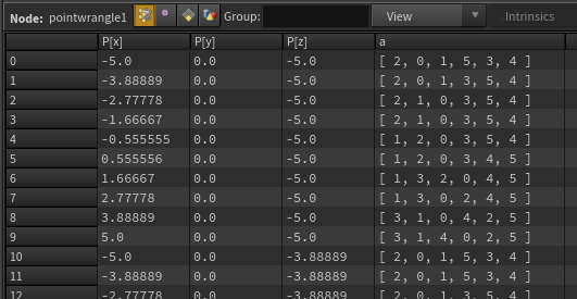
If I felt that was doing the right thing for my current task, I could then just delete or comment out that last line, and carry on.
Bonus tip! You can quickly comment/uncomment a line with ctrl-/
Nearpoints takes another optional value, the number of points to return. So to return points within 12 units, but limit the result to the closest 3 points:
vex
 int pts[];
 pts = nearpoints(1,@P,12,3);
int pts[];
pts = nearpoints(1,@P,12,3);Similar to getting the length of a vector with length(@P), you can get the length of an array with len. This just counts the number of items in the array. We could use this to do some cheap terraforming, by setting P.y to the number of points found. Here I'll add sliders for the distance to search and the number of points to return:
vex
 int pts[];
 pts = nearpoints(1,@P,ch('radius'),chi('numpoints'));
 @P.y = len(pts);
int pts[];
pts = nearpoints(1,@P,ch('radius'),chi('numpoints'));
@P.y = len(pts);
Waves again
Now you know we can't get through a chapter without waves.
Lets do the usual setup; get the distance to the closest point and store it as d, generate waves with sin(d), and add some controls so we can control the frequency and height of the waves. Here I setup a new variable, w, where I do most of my calculation, and try and leave d untouched, so I can use the original distance calculation again at the end:
vex
int pts[];
int pt;
vector pos;
float d,w;

pts = nearpoints(1,@P,ch('radius'),chi('number_of_points'));

pt = pts[0];
pos = point(1,'P',pt);
d = distance(@P, pos);
w = d*ch('freq');
w -= @Time * ch('speed');
w = sin(w);
w *= ch('amp');
w *= fit(d,0,ch('radius'),1,0);
@P.y += w;
int pts[];
int pt;
vector pos;
float d,w;
pts = nearpoints(1,@P,ch('radius'),chi('number_of_points'));
pt = pts[0];
pos = point(1,'P',pt);
d = distance(@P, pos);
w = d*ch('freq');
w -= @Time * ch('speed');
w = sin(w);
w *= ch('amp');
w *= fit(d,0,ch('radius'),1,0);
@P.y += w;It looks like a lot, but its all made of steps we've done so far. Stepping through the lines, we initialise our variables, and create the pts array. Then we grab the closest point, get its position, and measure the distance from our grid point to the scattered point.
If we fed this value directly to sin, we'd get a very wide wave. By multiplying this distance, we make the sin function generate tighter waves.
Of course we want this to animate, so it gets multiplied by @Time, which itself is multiplied by a speed value.
Then we do the sin function, which makes w a wave between -1 and 1.
That will be too big for the fine ripples I have in mind, so I multiply it by ch('amp') to bring it down to the scale I need, probably around 0.2.
If we fed this result to P.y, the waves are all the same height, no matter how far away they are from the scatter points. Ideally we want the wave height to decay the further away they are from the scatter points. And thats why I keep the d value safe, this is the exact value we need for this last step! The only problem is that it will be 0 where the wave starts, and gradually increase, but we want it to be 1 where the wave starts, and reduce to 0 at the maximum ripple distance, so a fit is used to invert and scale the value.
Finally that's applied to P.y. By adjusting the sliders (and adding lots more divisions to the grid), I get this:

Thats ok, but even though the fade almost hides it, the waves are still being clipped at the cell borders. But look what happens if I set the 'pt = pts[0];' line, which works with the nearest scattered point to every point on the grid, to 'pt = pts[1];', ie, the second nearest point:

That's the missing falloff we need! So to combine these two things, we can do a similar trick to earlier, just run the process twice, once for each point. Just remember that when you assign it to @P.y, that you add it ( += ) rather than just assign ( = ).
vex
int pts[];
int pt;
vector pos;
float d,w;

pts = nearpoints(1,@P,ch('radius'),chi('number_of_points'));

pt = pts[0];
pos = point(1,'P',pt);
d = distance(@P, pos);
w = d*ch('freq');
w -= @Time * ch('speed');
w = sin(w);
w *= ch('amp');
w *= fit(d,0,ch('radius'),1,0);
@P.y += w;
pt = pts[1];
pos = point(1,'P',pt);
d = distance(@P, pos);
w = d*ch('freq');
w -= @Time * ch('speed');
w = sin(w);
w *= ch('amp');
w *= fit(d,0,ch('radius'),1,0);
@P.y += w; int pts[];
int pt;
vector pos;
float d,w;
pts = nearpoints(1,@P,ch('radius'),chi('number_of_points'));
pt = pts[0];
pos = point(1,'P',pt);
d = distance(@P, pos);
w = d*ch('freq');
w -= @Time * ch('speed');
w = sin(w);
w *= ch('amp');
w *= fit(d,0,ch('radius'),1,0);
@P.y += w;
pt = pts[1];
pos = point(1,'P',pt);
d = distance(@P, pos);
w = d*ch('freq');
w -= @Time * ch('speed');
w = sin(w);
w *= ch('amp');
w *= fit(d,0,ch('radius'),1,0);
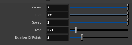
@P.y += w;Here's the settings I'm using to get these waves if you want to try and match:
Exercises
- Make this extend beyond to more scatter points by manually copying and pasting
- Make the waves include and mix colour
- Do different speeds and amplitudes for each wave hit (hint, you'll need to add a random amount to w somewhere, driven from pt)
prev: JoyOfVex11 this: JoyOfVex12 next: JoyOfVex13
main menu: JoyOfVex