Appearance
Joy of Vex Day 20
pointclouds, further learning
Pointclouds
In a similar way that minpos is the 'simple' and primuv + xyzdist are the 'versatile' versions of the same thing, it helps to think of nearpoint and nearpoints as the simple version of the more advanced pointcloud collection of vex functions.
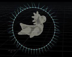
To show how similar they are in the simple case, start with what we had yesterday; single point to first input of a wrangle, 10x10 grid to the second input, we'll look up the nearest points to the single point, and create new points there. The function expects you to tell it which geo input to look at, the position to start from, and optionally the maximum distance to search and maximum number of points to return.
vex
 int pts[] = nearpoints(1,@P,ch('d'),25);
 int pt;
 vector pos;
 foreach (pt; pts) {
   pos = point(1,'P',pt);
   addpoint(0,pos);
 }
int pts[] = nearpoints(1,@P,ch('d'),25);
int pt;
vector pos;
foreach (pt; pts) {
pos = point(1,'P',pt);
addpoint(0,pos);
}
Now look at the equivalent pointcloud version:
vex
 int pts[] = pcfind(1,'P',@P,ch('d'),25);
 int pt;
 vector pos;
 foreach (pt; pts) {
   pos = point(1,'P',pt);
   addpoint(0,pos);
 }
int pts[] = pcfind(1,'P',@P,ch('d'),25);
int pt;
vector pos;
foreach (pt; pts) {
pos = point(1,'P',pt);
addpoint(0,pos);
}It's almost identical! The only difference is that pcfind doesn't let you optionally set the max dist and max points, they're required.
So in a simple case like this, nearpoints is probably better. Lets try some more advanced stuff.
Average position
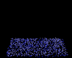
A handy feature of point clouds is the ability to filter or average values. Easier to understand with a few counter examples, then see what pointclouds can do. Bit of setup for this one, but its worth it. Create a rubber toy, a open arc poly circle that is on the YZ plane, about 50 points, and append a transform sop to the circles so that it rotates slowly on the x-axis, say @Time*3. The aim is to get a slow carousel of points that circle around the rubber toy:
Connect the circle to the first input of a point wrangle, toy to the second (make sure to template display the toy so you can see what's going on).
First thing we'll do is snap the points of the circle to the closest position on the toy. minpos can do that:
vex
@P = minpos(1, @P); @P = minpos(1, @P);
That works, but its a pretty steppy. Ideally we'd get @P from many points, add them up, average them. That should smooth things. Lets do that with nearpoints:
vex
 int pts[] = nearpoints(1,@P,ch('d'),chi('amnt'));
 int pt;
 vector pos = 0;
 foreach (pt; pts) {
   pos += point(1,'P',pt);
 }
 @P = pos/len(pts);
int pts[] = nearpoints(1,@P,ch('d'),chi('amnt'));
int pt;
vector pos = 0;
foreach (pt; pts) {
pos += point(1,'P',pt);
}
@P = pos/len(pts);Set the 'd' slider to 10, and keep pushing the amnt slider to from 10, to 100, to 500, 1000, and you'll see the circle conform to an ever smoother shape:
That's all well and good, but we can do that in 2 lines with pointclouds:
vex
 int mypc = pcopen(1, 'P', @P, ch('d'), chi('amnt'));
 @P = pcfilter(mypc, 'P');
int mypc = pcopen(1, 'P', @P, ch('d'), chi('amnt'));
@P = pcfilter(mypc, 'P');This first line sets up a pointcloud, and uses the same distance and number of points inputs as the nearpoints function. Pcopen returns a temporary handle to this pointcloud, similar to the way '0' or '1' refers to the input geometry, this is an integer that refers to 'a thing', in this case the pointcloud we just created.
The second line calls pcfilter, which when given the pointcloud handle we just generated, automatically does the sum+average trick we just did manually with nearpoints.
What's cool about this is you can get it to average any attribute from the pointcloud. Eg, the average normal:
vex
 int mypc = pcopen(1, 'P', @P, ch('d'), chi('amnt'));
 @N = pcfilter(mypc, 'N');
 @N = normalize(@N) *2;   // to make it easier to see!
int mypc = pcopen(1, 'P', @P, ch('d'), chi('amnt'));
@N = pcfilter(mypc, 'N');
@N = normalize(@N) *2; // to make it easier to see!Again, winding the number of points from 10 to 100 to 1500, you can see the normals get smoother and smoother:
Blurred colour
The trick I used to do with this a lot was to blur colour. Here I've got a 200x200 grid, an attribfrommap sop, and the following wrangle. Unlike the previous example, this one refers to input 0, ie its blurring itself, rather than doing it relative to another input geo:
vex
 int pc = pcopen(0,'P',@P, ch('dist'), chi('maxpoints'));
 @Cd = pcfilter(pc, 'Cd');
int pc = pcopen(0,'P',@P, ch('dist'), chi('maxpoints'));
@Cd = pcfilter(pc, 'Cd');Pushing the maxpoints slider to 10, 100, 100, 2000 etc gets pretty blurry:
These days I mainly just use a attrib blur sop, but this is a fun vex trick.
Use lookups other than P
Going off the deep end here of pointcloud tricks you may never use, but now you can stick it in the back of your mind for one day...
Just to re-iterate what we've been doing here; each time we run these point cloud functions, we're creating a list of the closest points to the current point we're working with. That list can be quickly sorted and queried to lookup some attribute.
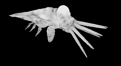
But think about that 'closest points' bit of the description. We've been getting the closest point in terms of position. But it doesn't have to be. Instead we could return points that are the closest in colour, then lookup attributes on that result (this is a plane, attribfrommap using Mandril.pic, converted to points):
vex
 int pc = pcopen(0,'Cd',@Cd, ch('dist'), chi('maxpoints'));
 @P = pcfilter(pc, 'P');
int pc = pcopen(0,'Cd',@Cd, ch('dist'), chi('maxpoints'));
@P = pcfilter(pc, 'P');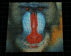
What's going on in the above gif is each point gets a pointcloud of all the points that are nearest in colour, then using pcfilter get the average position of those points. This has the effect of all similar coloured points start moving towards their average center. You can see all the red bits of the nose collapse together, as do the blue, and the general greeny brown fur tries to tend towards the average, but its so wide that it just gets pushed into a weird smudge. Interesting but useless, my favourite kind of vex trick.
Same cool but useless trick of looking up points that match on nearest @N, then move to the average position of those points on a heavily subdivided pig. Why? Because! (Make sure the pig has point normals):
vex
 int pc = pcopen(0, 'N', @N, ch('dist'), chi('maxpoints'));
 @P = pcfilter(pc, 'P');
 @Cd = @N;
int pc = pcopen(0, 'N', @N, ch('dist'), chi('maxpoints'));
@P = pcfilter(pc, 'P');
@Cd = @N;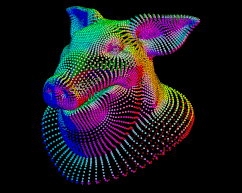
pop sim and pointclouds
Download scene: pc_popforce.hipnc
Slightly less silly example, one I half-remembered from an odforce post that I didn't understand when I first saw it, sort of understand now.
I have a wobbly tube that has @v swirling around it courtesy of a polyframe, and a grid that emits particles. The particles are using a pc lookup to get the average blurred v and P from the cylinder, and use it to calculate their own velocity (input 1 to the popnet is the tube)
vex
 int pc = pcopen(1,'P',@P,10,30);
 vector avgv = pcfilter(pc,'v');
 vector avgp = pcfilter(pc,'P');
 avgv *= {1,0.1,1};
 avgp *= {1,0.1,1};
 @v += avgv-avgp;
int pc = pcopen(1,'P',@P,10,30);
vector avgv = pcfilter(pc,'v');
vector avgp = pcfilter(pc,'P');
avgv *= {1,0.1,1};
avgp *= {1,0.1,1};
@v += avgv-avgp;The result is a smooth vel force that somewhat conforms all the particles to move together. An even more interesting result can be had by emitting from the tube, and pointing pcopen at the particles themselves (ie, pcopen(0, 'P' etc ) ; local variation in the particles gets cancelled out, they start to clump almost like stars in galaxies. Set the number of points to return high enough it gets very slow, but even bigger more stable clumps form.
Ambient Occlusion
Download scene: pbao.hiplc
Not quite AO, but it'll do. The idea here is to lookup a blurred position, or blurred normal via a point cloud, then get a pseudo AO look by either comparing a dot product of the real N and blurred N, or the distance from the real P to blurred P. The result is really more of a curvature/density map than AO, but gives an idea of what's possible.
vex
int pc = pcopen(0, "P", @P+@N*ch('bias'), ch('maxdist'), chi('numpoints'));

vector pcp, pcn;
float dot, dist;

pcp = pcfilter(pc, 'P');
pcn = pcfilter(pc, 'N');

dot = dot(@N, pcn);
dist = distance(@P, pcp);

dot = chramp('dot_cc',dot);
dist = chramp('dist_cc',dist);

@Cd = dot;
//@Cd = dist;
int pc = pcopen(0, "P", @P+@N*ch('bias'), ch('maxdist'), chi('numpoints'));
vector pcp, pcn;
float dot, dist;
pcp = pcfilter(pc, 'P');
pcn = pcfilter(pc, 'N');
dot = dot(@N, pcn);
dist = distance(@P, pcp);
dot = chramp('dot_cc',dot);
dist = chramp('dist_cc',dist);
@Cd = dot;
//@Cd = dist;Patreon supporter Laurent Menu wrote in with some great feedback:
I would use an abs() to avoid the dot product to return negative values (I tried on Crag and the colors were like stripes around cavity areas).
And a bit later with some full example code, where he dropped the abs, but used a fit to get the full range of values from the dot product. I took that one more step and ran it through a gamma/pow function to increase contrast:
vex
int pc = pcopen(0, "P", @P, ch('maxdist'), chi('numpoints'));
vector pcn = normalize(pcfilter(pc, 'N'));
vector norm = normalize(@N);
float dot = dot(norm, pcn);
@Cd = fit(dot, -1, 1, 0, 1);
@Cd = pow(@Cd, ch('gamma'));
int pc = pcopen(0, "P", @P, ch('maxdist'), chi('numpoints'));
vector pcn = normalize(pcfilter(pc, 'N'));
vector norm = normalize(@N);
float dot = dot(norm, pcn);
@Cd = fit(dot, -1, 1, 0, 1);
@Cd = pow(@Cd, ch('gamma'));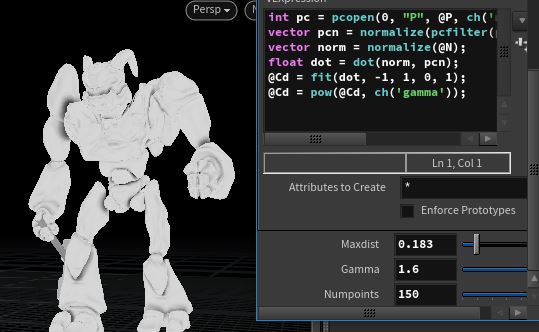
Again, not proper AO, but looks pretty good. Thanks Laurent!
Exercises
As I said earlier, I don't use pointclouds much, so struggling to think of exercises... if you can suggest some, get in touch!
Congratulations
You've made it! Where to from here? What haven't I covered?
Well, lots actually. I only vaguely touched on vex in dops, there's also volume wrangles, inline vex in vops, vops in cops, chops, materials, and probably several other places I don't know about. That said, vex is fairly consistent across different contexts, and there's usually some example code either within sidefx nodes, or the help, or the forums to get you started.
If you're interested in more gifs and words, you can probably handle the HoudiniVex1 page now. In fact you'll find you can probably skip the first 10 or so chapters, which were a compressed and hastily written version of these tutorials.
In fact if you browse around the wiki pages you'll find I have vex examples on most pages. Again, they should now all be much less daunting now, but if you find any repeated patterns in my vex examples that I haven't explained in these 20 days, let me know.
External links
- If you want a more structured and thorough guide to Vex, Juraj Tomori has written a fantastic guide: https://github.com/jtomori/vex_tutorial
- Entagma are also doing a Vex introduction course, their material is always fantastic: https://www.patreon.com/entagma/posts
- Check this incredible tutorial by Kiryha! https://github.com/kiryha/Houdini/wiki/vex-for-artists
If you know of other resource links I should put here, again, please get in touch.
This whole thing took a LOT more time and effort than I anticipated. If you wanna say thanks, click that Patreon link below. 😃
-matt
prev: JoyOfVex19 this: JoyOfVex20 next: VexCheatSheet
main menu: JoyOfVex